This post is part of a series of paper reviews, covering the ~30 papers Ilya Sutskever sent to John Carmack to learn about AI. To see the rest of the reviews, go here.
Paper 15: Neural Machine Translation by Jointly Learning to Align and Translate
High level
Ah, the attention paper. It's hard to overstate how incredibly important this paper is to the ML canon. Attention has come up repeatedly in the papers we've reviewed thus far; here, we see its origins.
Back in 2015, folks were using LSTMs to model language. An LSTM would ingest words in a sequence one by one. For each word, the LSTM would update some embedding representation. And then some other sequence generator (often also an LSTM) would take that embedding representation and sequentially produce some output.
In the past I’ve emphasized the importance of embeddings and thinking about what embeddings actually represent. Architecture matters a lot here — the structure of a model has a direct impact on how data gets written to or erased from some set of embeddings. In the case of a standard seq2seq model, the LSTM is learning prefix embeddings. That is, each stage of the LSTM has to capture all of the data that came before it.
Funny enough, I wrote about this exact problem previously in the LSTM blog post review:
As the [RNN] processes each element in the sequence, it can learn a representation of the prefix (the data it has seen thus far) which can guide how it processes the next step.
…
RNNs in their most basic form — a single loop — have a big problem. The model doesn't "know" what information it might need at each future step. So, as a sequence gets longer, the model has to pack more and more information into the 'message' that is passed from one time step to the next. But it only has a fixed vector size with which to do so, and there is a limited amount of computation capacity in the single layer of weights that are used to update the state. At some point, the model runs into information theoretic limits. This in turn makes it hard to represent long range dependencies.
In that review, I discussed how LSTMs improve the ability to handle long-range dependencies. But it's not a permanent fix, and as models scaled up more the prefix-learning problem reared its head again. And so we get to the central motivation of the attention paper in the first place. From the paper:
A potential issue with this encoder–decoder approach is that a neural network needs to be able to compress all the necessary information of a source sentence into a fixed-length vector. This may make it difficult for the neural network to cope with long sentences, especially those that are longer than the sentences in the training corpus.
The authors propose a method to figure out what information matters for each word dynamically, thereby bypassing the information compression issue.
We start with an “attention” function. Generally, the attention function takes in two vectors and produces some number that represents a 'weight'. Often, that weight can be interpreted as a 'similarity'. In the paper, the attention function is a learned neural network that takes in some representation of each word (more on this in a second) and the current decoder hidden state and produces a vector of weights.1 The model runs a softmax over the attention vector, multiplies the word-representations by the corresponding attention-weights and adds them all together to get a final 'context' vector.2
How do we actually get these word vectors?
One naive approach is to just run an RNN over the sequence and take the hidden state of each step as the corresponding representation for the word at that part of the sequence. But this runs into a variant of the same 'prefix' problem we mentioned earlier. The hidden state for the last word will have information about the whole sentence, while the hidden state for the first word will have none. More generally, the authors want the hidden state for each word to represent information on both sides of the sentence.
The trick is to simply run two RNNs. They run one RNN forward over the sentence and one backwards. For each step, they concatenate the two hidden states together to produce one 'word' vector. The forward running hidden state will have all of the information up till that point, x0 - i. And the backwards running hidden state will have all of the information after that point, xi - n.3

One last note on architecture: beam search.
It may be weird to think about it this way, but language modelling is best thought of as a categorization task. Given some input, the model has to predict which of N categories is the most likely output. It's just that for language modelling, there are a lot of categories — one for each token, to be precise. As with all categorization tasks, the model does not output a single value. Rather, it outputs a probability distribution that represents the model's confidence of the output.
The authors are interested in text-translation, a subset of language modeling. They have some input text and they are trying to produce some output text. For each word, the model produces a probability distribution. If the output has 10 words, the model is actually producing a [10, N] matrix, where N is the number of tokens. We need to turn these into words somehow.
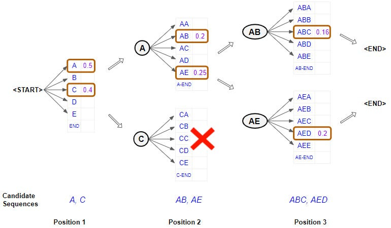
Naively, you could turn each probability distribution into a single word by simply looking at the largest value in that particular distribution. But this may lead to worse outcomes over the whole probability distribution (i.e. the whole sentence). For example, imagine you wanted to translate ‘quick brown fox’. The model may output ‘maroon’ instead of ‘brown’ as the most likely translation for the second word, which makes it much less likely to output ‘fox’ as the third word.
So the naive option has pitfalls. On the other extreme, you could try to maximize the probability of the entire sequence by looking at every combination of words. This is a NS operation, where N is the number of possible tokens and S is the sequence length. It's way too expensive.
So the authors use a technique called beam search. Instead of greedily choosing one word at a team, beam search aims to maximize the probability of phrases over the whole sentence. It's more accurate than simply running greedy, but less costly than doing a full search.

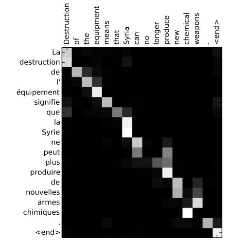
During experiments, the authors show a higher BLEU score on their translations, especially for longer sequences.4 They also show attention alignment results — they get some very cool graphs showing how their ‘attention model’ decides which words are important to which output words depend on which input words.
Even today, these sorts of graphs are the bread and butter of understanding what exactly language models are doing.
Insights
I tend to come at things from a representation learning perspective. The thing I'm generally thinking about when evaluating a deep learning architecture is "what, exactly, is this model learning?" It's not immediately obvious that Seq2Seq models learn prefix embeddings, but once that clicks all of the limitations of a traditional LSTM become immediately clear.
So from a representation learning perspective, the main innovation of this paper is the switch from learning sentence prefix embeddings to learning word embeddings and a reduce operation. Or, more generally, from learning sequence prefixes to learning set element representations. This is a powerful change. Prefixes are inherently unbounded, as a set increases in size so does the amount of information that a prefix embedding needs to store. That in turn means that a prefix embedding of a fixed size will lose resolution as the input gets larger. By contrast, word embeddings store a roughly constant amount of information. With attention, any set of weights within the model has to learn fewer things, and the overall complexity of what needs to be represented in any given embedding drops dramatically.
The attention mechanism is particularly elegant as a solution to the capacity problem, because it's not structurally limited to any particular kind of input information or problem space. In this paper the authors apply attention to learning word embeddings, but you could just as easily apply the general principles of attention to sentences, images, video…basically any kind of data. The reason attention is so flexible is because it is fundamentally a latent operation. It operates on embedding representations, which are essentially type-less. And as we've discussed in the past, attention in particular is also order invariant, which immediately makes it useful outside of sequential settings.
Other than that, the attention paper fits in with two larger patterns that we've seen across these papers.
First, information bottlenecks are bad. This is something we saw in both the ResNet paper and the LSTM blog post. If your model architecture requires all of your data to be funneled through a single stage, your model's representation capacity is effectively capped by the size of that stage.
Second, models seem to do better when you separate "operations" from "representation". This was something we discussed in depth in the identity mapping paper. It's not clear exactly when a particular set of weights is a representation and when it is an operation, but there's something there.
One last thought.
Attention at a micro level operates very similarly to the way people think about context and context windows at the macro level of LLMs today. One of the themes of the LLM Primer Series is that LLMs are pretty good at doing the right thing as long as they have context. Most of the challenge of LLMs is figuring out how to find and fit the right information into that context window. How do we find the right information? A lot of people turn to RAG systems that use some sort of similarity measure over a vector database to pull out and use key information.
But this is just attention! The RAG systems are implementing a larger form of attention over a bigger database, but that's all it is! Another way of framing this: attention is simply a vector search algorithm that is embedded within a model's weights. And as further evidence of this, the authors actually use search terminology.
Each time the proposed model generates a word in a translation, it (soft-)searches for a set of positions in a source sentence where the most relevant information is concentrated.
The new architecture consists of a bidirectional RNN as an encoder (Sec. 3.2) and a decoder that emulates searching through a source sentence during decoding a translation (Sec. 3.1)
That search terminology carries all the way through to Transformers, and is where we get the Query/Key verbiage from.
Note that since it’s a translation task, you actually do have the whole sequence of the input a priori, i.e. you can ‘attend’ to ‘future’ words.
The phrasing in the paper is interesting — they treat it as a ‘separate model’. There was an era of ML where it was popular to talk about large ML models as if they were composed of smaller models. Often these papers would talk about “joint training”. I think we’ve dropped that language as an industry. A jointly trained model is just a large model.
I recently saw Tenet, which is a movie that makes zero sense, but I found it surprisingly useful as a metaphor to understand what these RNNs are doing.
BLEU is a quantification for how good a translation is. I think it’s mostly fallen out of favor as a quantification method, but don’t quote me on that — part of the reason it may no longer be used is AI has simply solved translation to a high enough level that we can’t really get more use out of it as a metric.


