
Neural Architecture for Dummies
A no-math guide on how to break down and reason about neural network architectures

Deep learning does not have any formal theory. Instead, researchers build up intuition. A core part of intuition is thinking about what different model architectures and vector operations do. Not in a mathematical, 1s and 0s sense. But in a ‘network of operations’ sense. The folks who are the most talented at putting together models aren’t thinking in terms of linear algebra. They are one layer abstracted, thinking about flows of meaning and representation.
This article is my attempt to share some of that intuition. Each section of this article is dedicated to a single operation and how you might implement that operation using a neural network architecture. In part 2, I walk through a few examples of how to compose these operations into higher level circuits and models.
One note: training an ML model is like pouring water down a mountain of sand. You can control where the water goes by etching grooves into the sand, but rivers do not appear until the water falls. Similarly, at train start, the model is randomly initialized and the operations don’t ‘exist’ yet. But in the same way the valleys direct water, the architecture of the model ‘encourages’ learning specific operations/configurations during training. It’s a bit like gears and pipes in a big steampunk machine. We can analyze the mechanics of what the machine will do before we even turn it on. But you need to turn it on before the machine will do anything at all.
Operation: Assigning Variables to a Concept
Implementation: Matrix / Weight initialization
ML models represent the world using vectors. A vector is a list of numbers. All lists of numbers are just points in a coordinate space. So ML models represent the world as points in a coordinate space. Sometimes, we call these vectors ‘embeddings’ or ‘embedding vectors’. From my simple deep learning series:
Embeddings allow us to turn concepts into points in space, where we can visualize things like ‘distance’ or ‘surfaces’. When I think about creating a model to embed cars, I imagine a fantasy map where different regions represent specific car makes and models. You have a Mercedes town, which is pretty close to BMW-burg , and kinda far from the Bus-ville. If our map does a good job keeping similar things close to each other, we’ve solved 90% of the deep learning problem.
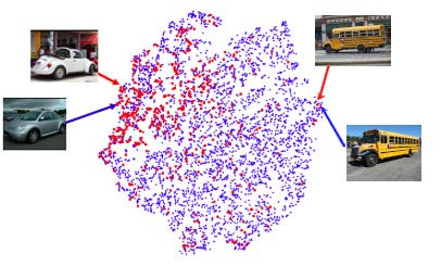
(see Simple DL for more)
In code, we often need to assign values to specific variables. For example, x = 5. In a neural net, we often need to assign values to a set of vectors. As it turns out, this is just a matrix initialization. Any weight matrix creates a unique assignment per row.
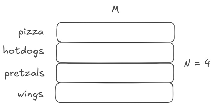
In the above image, N is the number of concepts you care about, and M is the length of the vectors assigned to each concept. You can think of M as the ‘representational capacity’ of the concepts. The larger M is, the more nuanced the concepts can be. If M is small, you may be able to represent car vs bus vs bicycle. If M is large, you may be able to get more nuanced, representing Mercedes and BMW.
Sometimes, these initialized representation matrices are called ‘vocabularies’, because they are often used in natural language models to represent vocabularies of words or tokens. For example, GPT3 learns how to represent a vocabulary of roughly 50k unique tokens. At the very start of the model architecture, we initialize a 50k x M matrix.1 You can think of this as 50k variable assignments. The 0th row is assigned to represent ‘the’. The 1st row is assigned to represent ‘that’. The 3724th row is assigned to represent ‘tree’. And so on.
Before any training occurs, these vectors are all random even though they are ‘assigned’ to specific tokens. The vectors themselves do not yet have any meaning, because the assignment only happens during training! As the model trains, it will adjust these internal representations until the individual rows in the vocabulary have distinct meaning. If the training is done correctly, the vectors will be represent the ‘meaning’ of that token. One important caveat: these vector representations are entirely defined by their relations to each other. You cannot take a vector from one place and read it easily in another place.
Operation: Combining Information
Implementation: Linear Vector Operations
Embedding vectors represent concepts, but they are also mathematical constructs, literally points in space. That means you can do math on these embedding vectors. Imagine you have two RGB “embedding” vectors that represent colors — [128, 0, 0] and [0, 0, 128], representing red and blue respectively. If you wanted to make purple, what would you do?
You’d add them.
Adding vectors is the same thing as combining information about concepts. If you add our red vector and our blue vector, you get [128, 128, 0], a purple vector. Colors are easy to reason about, but this logic works for arbitrary concepts. If you have a ‘happy’ vector and a ‘dog’ vector, adding them together creates a ‘happy dog’ vector.2
You can use scalar multiplication to increase the magnitude or ‘weight’ of how each concept is merged together. Going back to our colors example, if you want a blueish purple instead of regular purple, you could multiply the blue vector by 2 before adding them together: [128, 0, 0] + 2 * [0, 0, 128] = [128, 0, 256]. Or with our happy dog example, you could imagine a dog that is twice as happy.
Scalar multiplication is about increasing ‘how much’ of a concept ends up in the output. If you multiplied a ‘dog’ vector by 2, you are creating a representation of ‘more’ dog. This obviously will do weird things at the edges — you can’t multiply a vector by a billion and expect to get something coherent — so in practice we generally constrain linear vector operations to a tightly bound range.
Operation: Geospatial Composition
Implementation: Convolutions
Creating representation vocabularies for a model is really useful when you have a fixed number of non-numeric non-vector inputs, like tokens in sentences. The model doesn’t have any prior understanding of each token; the token is just a symbol. The model has to learn its own token-representation, and then learn how to process those representations.
This process doesn’t work as well for images, and for geospatial inputs in general. Geo-data has really strong and regular dependencies. Pixels relate to nearby pixels in consistent ways across all image dependencies. We often want to treat pixels (or voxels) differently based on their surroundings.
Convolutional layers are a pretty powerful abstraction. They work by sliding several ‘filters’ over sections of a grid / volume, and then producing an output at each section.
You can think of this as a way to identify geometric relationships. For example, if you know that dark pixels clustered together form boundaries, you can learn edge detectors. Or if you know that similar colored patches represent the same object, you can learn object detectors. Convolutions generally do not allow you to specify which specific euclidean relationship you are identifying. Rather, the output of the convolutional layer represents a mix of all of the relevant euclidean relationships that may exist.
Operation: Changing Resolution
Implementation: Convolutions
Surprise! Convolutions again!
As I said, convolutions are a powerful abstraction. In some models, it is best to think of them as identifying relationships between geometrically-dependent inputs. In other models, especially in models with many stacked convolutional layers, it is best to think of them as a mechanism to summarize information from one layer to the next, successively stripping things out and only retaining the most valuable pieces. This is why the individual convolutional weight matrices are called ‘filters’ — each one ‘filters’ some information out and keeps some other information in.
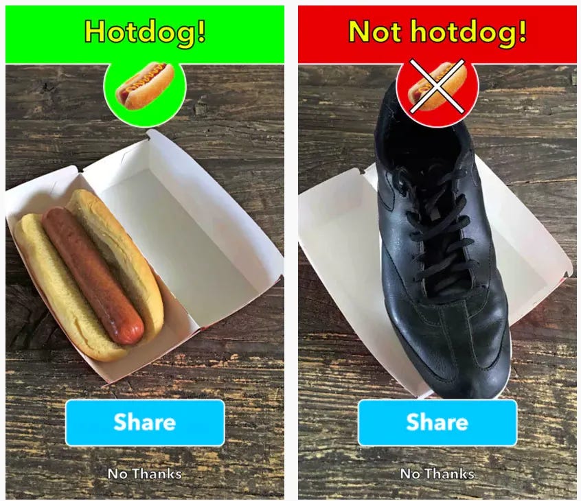
Convolutions summarize information based on proximity. That is, data that is located near each other in the underlying matrix is going to get bunched together and summarized. If you have random data near each other in your matrices, your summaries are not going to make any sense. But in geometric inputs (images, video, 3D models), we know that nearby information is very tightly related. In these settings, we can use stacked convolutions to summarize information, producing lower and lower resolutions. In the extreme, you can take something like an image and produce a single bit of information, like whether or not there is a hotdog in the image. Which, of course, is just doing binary classification on images.
Operation: Calculating Similarity
Implementation: Vector ✕ Vector
Let’s say I have two embedding vectors that both represent different concepts. I might want to calculate how similar these concepts are to each other.
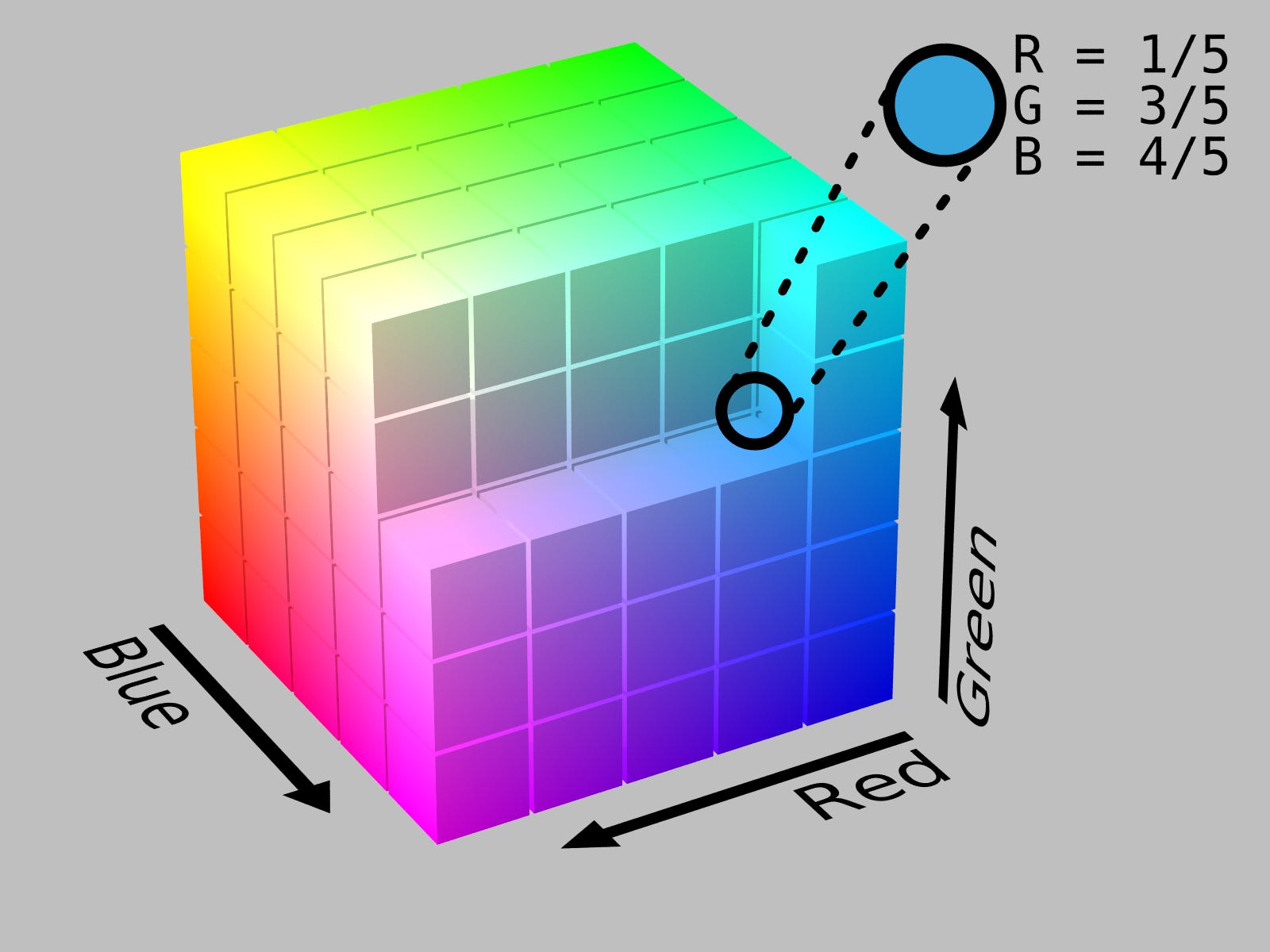
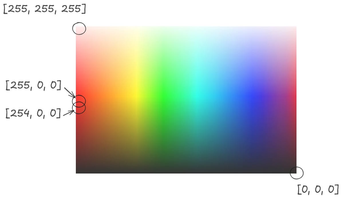
Assuming these vectors are in the same coordinate space, an easy way to quantify similarity is to measure the distance between these vectors. For some intuition, let’s again look at the color cube.
RGB vectors that are near each other — say [255, 0, 0] and [254, 0, 0] — are nearly indistinguishable. Vectors that are far from each other — say, [0, 0, 0] and [255, 255, 255] — look totally different.
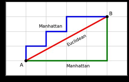
But what does “near” and “far” here mean? Well there’s a lot of distance / similarity measures3 that you can choose from. For example, you could sum the difference in values on each axis and add them together. This is called Manhattan Distance (because it’s like calculating distance on a grid of Manhattan blocks) or L1 distance. Or you could use Euclidean distance. This is the standard distance that we think about in 3D spaces, the shortest distance between two points calculated using something like the Pythagorean theorem. Euclidean distance is also closer to what we use for calculating distances between colors.
Or you could use cosine distance, which captures the size of the difference between the angles of the vectors.
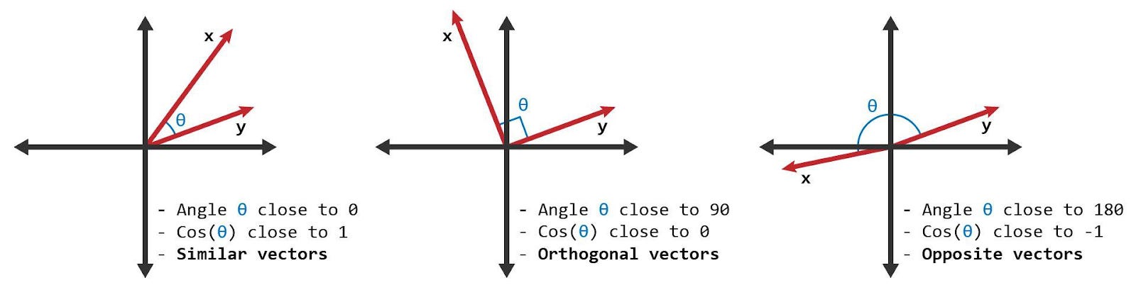
All of these are valid distance measures. In a defined vector embedding space, these measures approximate how similar concepts are. In a well defined vector embedding space, similar things will by definition be near each other.
Practically, it is very common to use cosine similarity as the similarity measure of choice, because it’s very easily represented as a vector * vector matrix multiplication.4 So whenever you see a vector being multiplied by another vector, you can think of the output as simply calculating some measure of similarity between those two vectors.
As a quick aside, distance measures that are calculated over sets of vector embeddings are the core of how vector databases work. Most vector databases implement an algorithm called kNN, or k nearest neighbors. For a given “query vector” and a distance operation, you calculate the distance of that vector against every other vector in the database. Smaller distances == more similar vectors. The output is a list of numbers that represent “similarity”, which you can then sort to find some number (k) nearby vectors. Remember, all of these vectors represent concepts. Sorting and selecting vectors is the same as finding the concepts in the database that are most similar to the input ‘query concept’.

Operation: Information Lookup
Implementation: One-hot vector ✕ Embedding Matrix
Let’s say we have a big embedding matrix of concepts. Each row corresponds to a particular concept or word. For example, row 1 may mean ‘the’ and row 1204 may mean ‘pizza’. Often you want to ‘pull out’ a specific concept or word in order to do more things with it.
You can do this with matrix multiplication. First, create a one-hot vector. A one-hot vector is vector with 0s everywhere, except one spot that has a 1. The one-hot vector should be as long as the number of rows in the embedding matrix. So if the matrix has 5 rows, the one-hot vector should have length = 5.
Then matmul that one-hot vector with the embedding matrix. The output is simply whichever row you set the 1 to in your one-hot vector. If you have a 1 in the 4th column, then you will get the 4th embedding vector row out of your matrix.
Here’s a visual depiction of how the linear algebra works out:
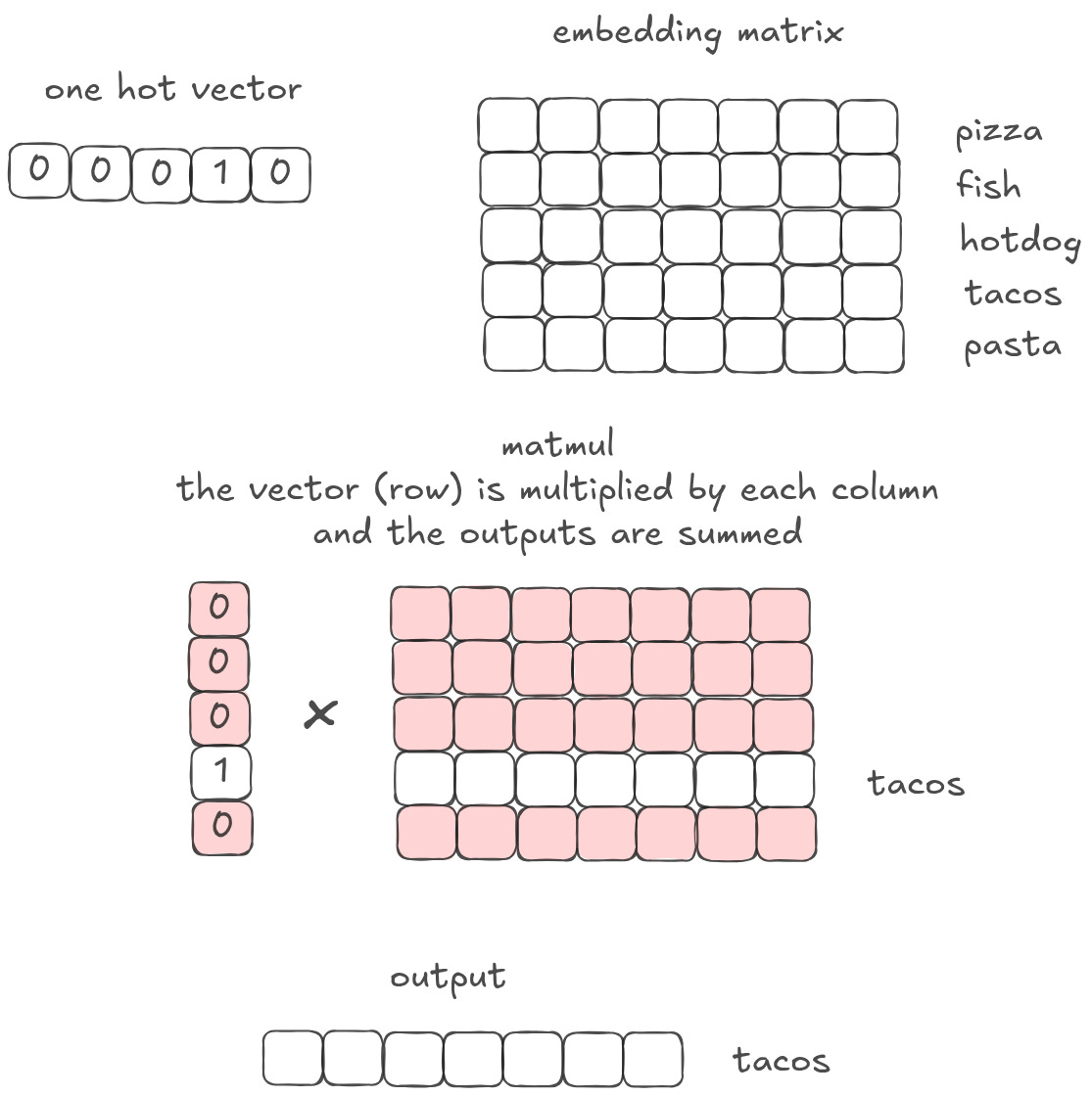
This is just an array indexing operation. You are using your one-hot lookup vector to ‘query’ a ‘database’ of other vectors.5 That database can be arbitrarily large. For example, it can be the size of the entire token vocabulary that a model is working with. The database can also store arbitrary information. Every matrix instantiation is essentially a bunch of variable assignments. In the example above, we assign each vector to a specific food. But in practice, those vectors could represent anything from paragraphs to documents to songs you may like on Spotify to potential matches on Hinge.
Operation: Weighted Summarization
Implementation: Vector ✕ Embedding Matrix
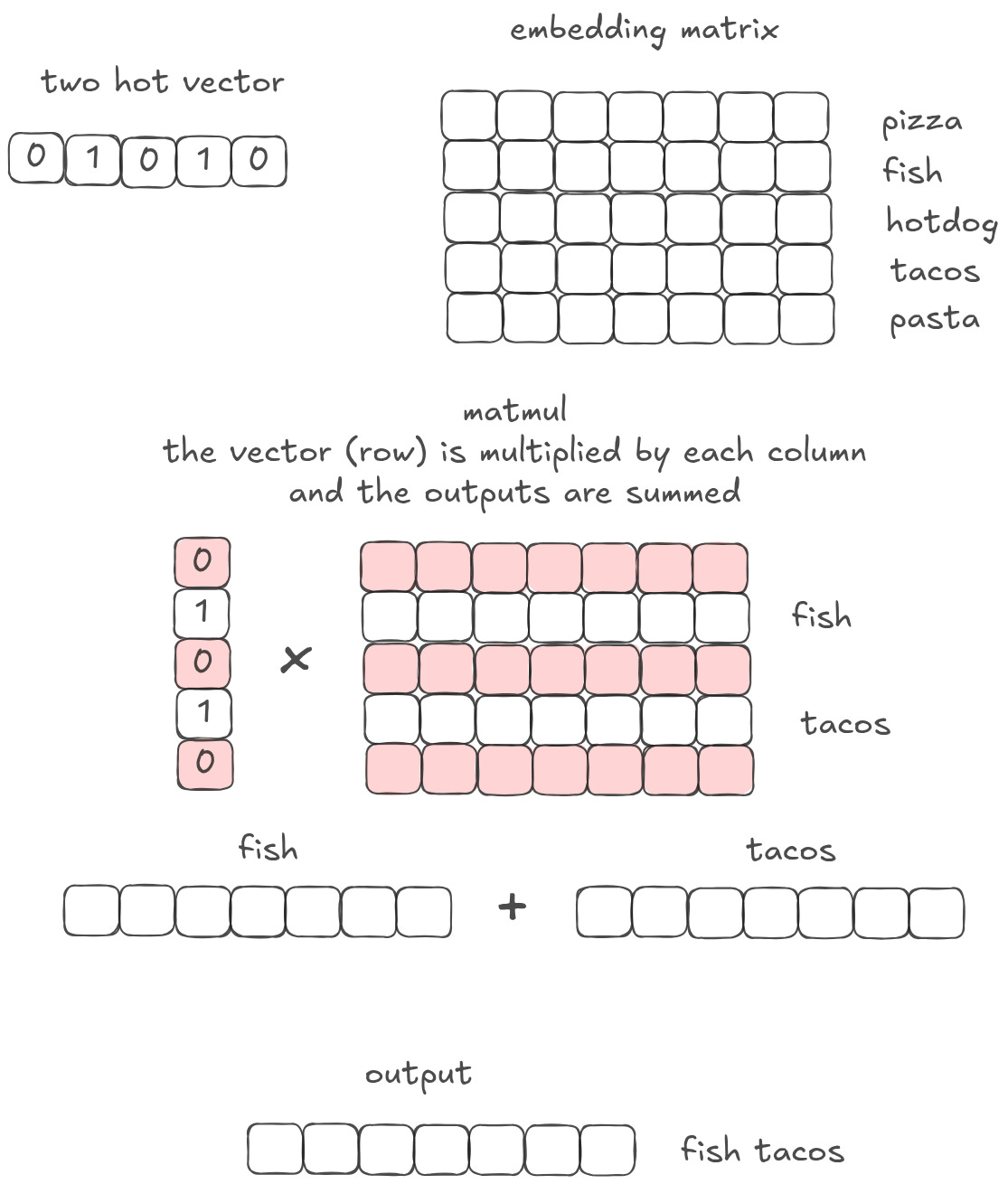
Let’s say instead of having a one-hot vector, you have a two-hot vector. It is a vector of 0s in every column, except a 1 in the second column and another in the fourth column. You then multiply your two hot vector by an embedding matrix. What comes out? In some sense, this is like doing a lookup twice. But that’s not quite right, because you only get one vector out on the other side.
Follow the linear algebra: when you do a matrix multiplication, you multiply the vector by each column, and then you sum the result. Remember what we said about summing vectors earlier? A sum is simply mixing two concepts together. So if I have a matrix multiplication with a two-hot vector, with a one on the ‘fish’ dimension and a 1 on the ‘tacos’ dimension, I will get a ‘fish tacos’ vector out. I do a lookup AND mixing in the same operation.
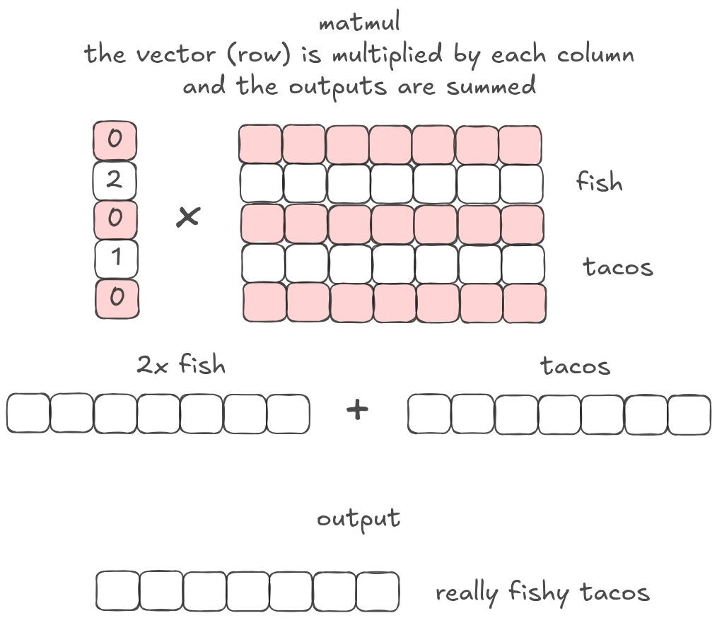
Let’s extend this a bit further. Instead of having a vector of just ones and zeros, I could have 2 and 1. Scalar multiplication is the same as changing the magnitude. So in this example, I would end up with fish tacos that are twice as fishy!
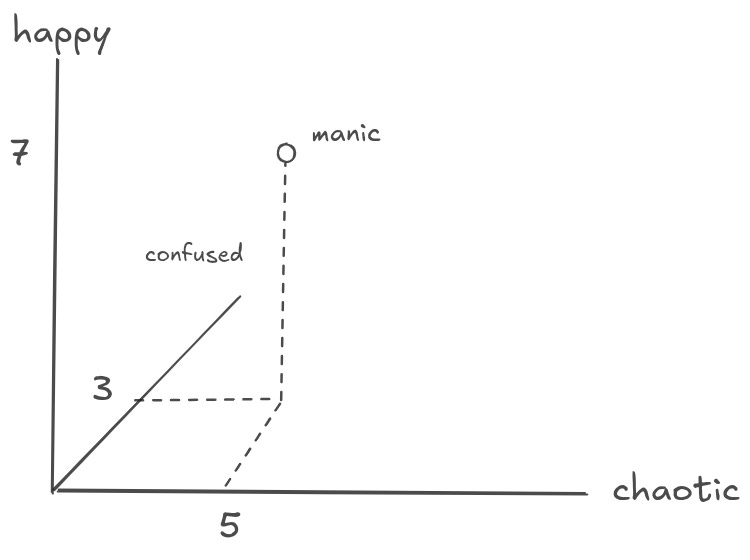
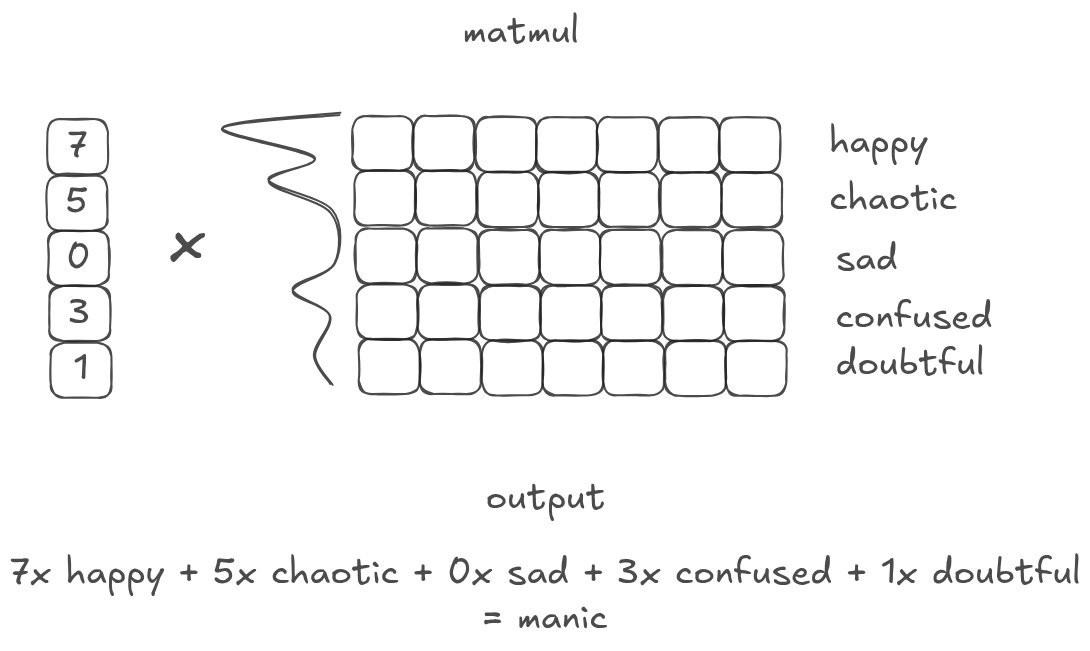
What if, instead of having only a few values, I have a vector full of different values? When I matmul that vector with a matrix of embeddings, I am collapsing all of the matrix representations into a single, weighted output. Or, in other words, I am creating a ‘weighted summary’ of the original matrix.6

What is an emotion or word that is 7 parts “happy”, 5 parts “chaotic”, 3 parts “confused”, and 1 part “doubtful”? ChatGPT came up with manic. Which, as a weighted summary of that database, isn’t actually that far off! Depending on what is important, you may weight the database differently to get different outputs that represent different things.
Operation: Change in representation
Implementation: Vector ✕ Embedding Matrix
A core part of making 3D games is placing objects in your game world. At a technical level, you have to tell your code what coordinate to place each object. But this is a funny question — coordinates relative to what? If I have a box at point [0, 0, 1], where is the box actually located? In most game engines, the box is given a coordinate that is relative to a fixed arbitrary [0, 0, 0] point. This is called ‘world space’. But then, when the game is actually being played, the engine needs to recalculate all of those locations relative to the position of the player’s camera. This is called ‘camera space’.

When you change from camera space to world space or world space to camera space, your directions change. In world space, xyz may correspond to horizontal/vertical/depth. If your camera is upside down and sideways, those all may be totally flipped!
How do you map from one space to the other? As it turns out, you just do a simple matrix multiplication. In linear algebra terms, this is a “change of basis.” Change of basis operations are a matmul between a vector and a ‘basis’ matrix. A change of basis does not actually change the underlying information stored in the vector. It simply changes how the vector is viewed.
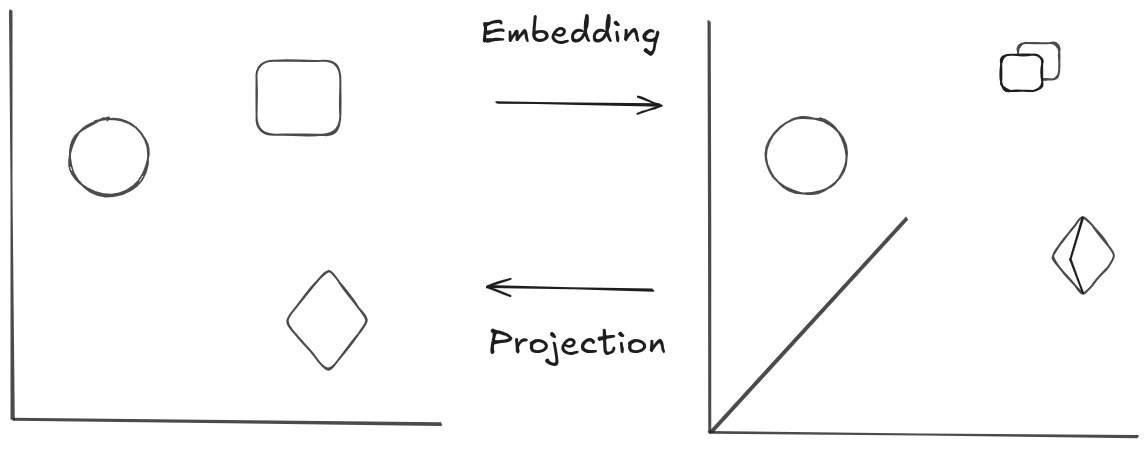
In deep learning terms, it’s helpful to think of this operation as a “change in representation” — that is, you are passing a vector through a matrix that (deterministically) maps that vector from one conceptual space to another. Your input vector is a point in some D dimensional space where each dimension has some meaning, and you transform it into a different coordinate space where the dimensions have different meaning. For example, let’s say you have a set of vectors that represent animals. You might pass these into a matrix that maps to emotions. So your “dog” vector might get mapped to “happy”, and your “cockroach” vector might get mapped to “disgust” and so on. Or, going back to our emotions example above, you can visualize the ‘change in representation’ by imagining each of those emotions as coordinate axes. The vector is then simply a point in the space defined by the emotions matrix.
You can generalize this concept to cases where you are adding and removing dimensions. In the former, you are “embedding” your vector in a higher dimensional space; in the latter, you are “projecting” it down to a lower dimensional space. And in the process of embedding up or projecting down, you can rotate the representation or “change its shape”.
This is the bread and butter of deep learning computation. It is the “generic” way to do “arbitrary” compute within a deep learning model. This is also, in a nutshell, what is happening inside a Dense layer.
Operation: Filtering
Implementation: ReLU
Any useful model will need to learn how to throw away information it does not need. Sometimes this is explicit in the task. If you are doing binary image categorization, you start with a very high dimensional, very dense pixel representation [height, width, 3 colors] and need to compress that down to one bit of information (hotdog, not hotdog).
One way you can do this compression is to simply decrease the size of your representation vectors. Above, we discussed how matrix multiplications are a “change in representation” operation. It’s reasonable to think that we could “change our representation” to remove some information. Going back to our emotions matrix, we can just set some of the emotions to 0 and that information will no longer show up.
In practice, there is a problem here — it is very difficult for a model to set any weight to 0 just by changing representations. So in most cases, every bit of information in the input will have some impact on the output. More broadly, in a standard multi-layer perceptron, the model is only able to add information together (after all, a matmul is “just” a weighted addition of a bunch of vectors). The model can’t easily forget anything as the data passes through the layers, it has to pack all the information into increasingly small vector spaces.
This is where activation functions come into play. One way to think about activations is that they give a model the ability to selectively and contextually forget information. The most explicit example of this behavior is the ReLu function, which will drop all negative values to 0.
 - MachineLearningMastery.com")
One way to think about the ReLU function is that it increases the target area where data is forgotten. Because the target area is bigger, it is easier for the model to forget things. With ReLU, information that “isn’t useful” can be much more easily forgotten, allowing “useful” information to fill the rest of the space and propagate up through the model with less noise.
ReLU also impacts the gradients that flow through the model. If some information gets knocked out due to a ReLu, the gradients for that piece of information get knocked out too. So the model does not adjust to that input — or, put another way, the output classification will be invariant to that kind of information.
A common way to think about non-linear activation functions is that they allow a model to learn more complex functions. A model that is composed of only linear functions can only learn a linear function. A stack of linear layers is, in theory, equivalent to one linear layer — the model is essentially just learning a line to split categories. Activation functions change that. They allow a model to learn “bends” and “curves”.


On face the ‘bend and curve’ model of activation functions may seem unrelated to the ‘filter’ model of activation functions, but I think there’s actually a fairly deep link between these two intuitions. By default, all neurons are “on”, all the time. ReLU’s filtering behavior (only passing positive signals) creates breakpoints in the input space where activations turn off. These breakpoints divide the space into regions where different neurons (and therefore different linear transformations) are active. The result is a piece-wise linear function:
Within each region, the model behaves like a simple linear classifier.
Across regions, the filtering (on/off behavior of ReLU) allows the model to combine these linear pieces into a complex, curved boundary.
In the examples above, the ReLU function allows our models to learn conditions. “If the input is 4, filter out the first and third term, but keep the second term”.
Operation: Sort
Implementation: Softmax
Sometimes, you might want to rank how important different representations are. For example, you may want to find the vector with the ‘most’ similarity to another vector. Or you may want to calculate which of several output classes is the ‘most’ likely. These rankings have two important properties. First, they are zero-sum. When one value becomes higher, we want all other values to become lower. This should hopefully make some intuitive sense — in a traditional sorting algorithm, moving a value to the front implicitly means every other value has to move one step back. Second, they are comparable. You can look at two ranked things and understand how they relate to each other in the ranking.
In an embedding vector, the dimensions have specific meaning, so you can’t actually sort the values in the vector. You would jumble up your representation and get an output that is totally meaningless. Instead, you can use a softmax function. The softmax will convert the raw values in your vector into a set of positive numbers that sum to one, effectively turning arbitrary scores into a probability distribution that ranks each option by its relative importance and makes it easy to compare values against each other.
One interesting note: if you put a sort operation on top of a weighted summarization operation, you end up with a lookup operation!
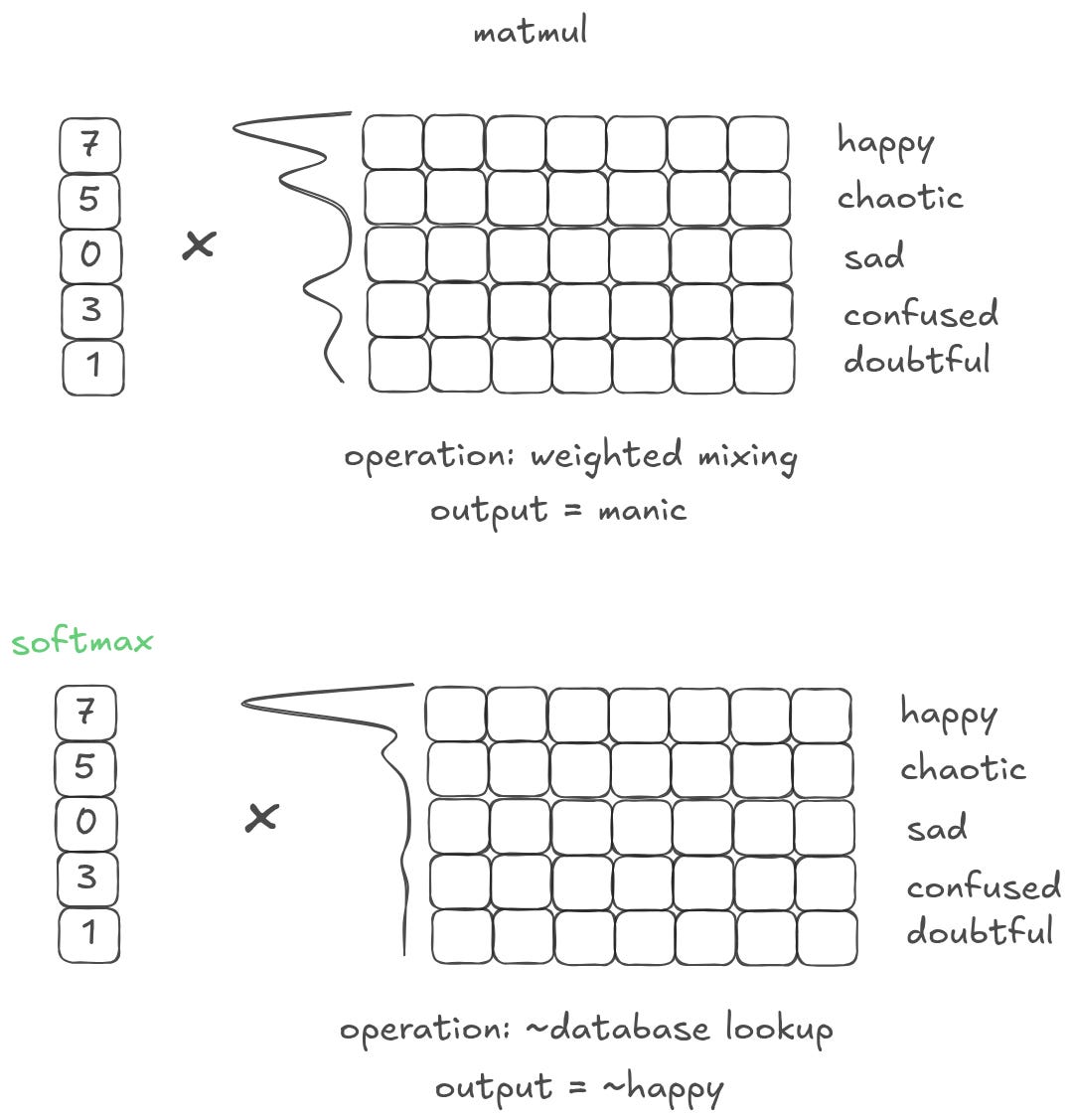
This is an extremely common pattern because it is the only way to get something that looks like an information lookup in real settings. We already discussed that actual models will rarely output zeros. This is structural — most of the time a model is inclined to provide a spread of values with all kinds of different weights and scales. Softmax is critical for forcing models to make tradeoffs between things. By wrapping a vector with a softmax, you drive the model towards an N-hot structure.
Operation: State
Implementation: Residuals
In a traditional software system, you need some way to store data for later use. At the most basic level this takes the form of variables and parameters; in more complex systems, its databases and disk. Generally, we call this ‘state’. State has two key properties:
The same “location” of state can take on many different kinds of values depending on the needs of a program;
The value of a piece of state does not change unless a program explicitly makes a change.
State is critical for basically any programs that are worth anything. In fact, state is so valuable that there’s an entire set of applications that are defined exclusively by their relationship to state — CRUD apps.
By default, a neural network has no state. Each layer takes in some input signal and outputs some transformation of that signal. There is no abstraction between the storage medium and the data.
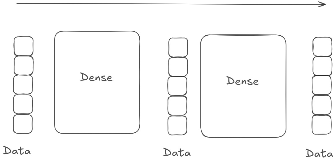
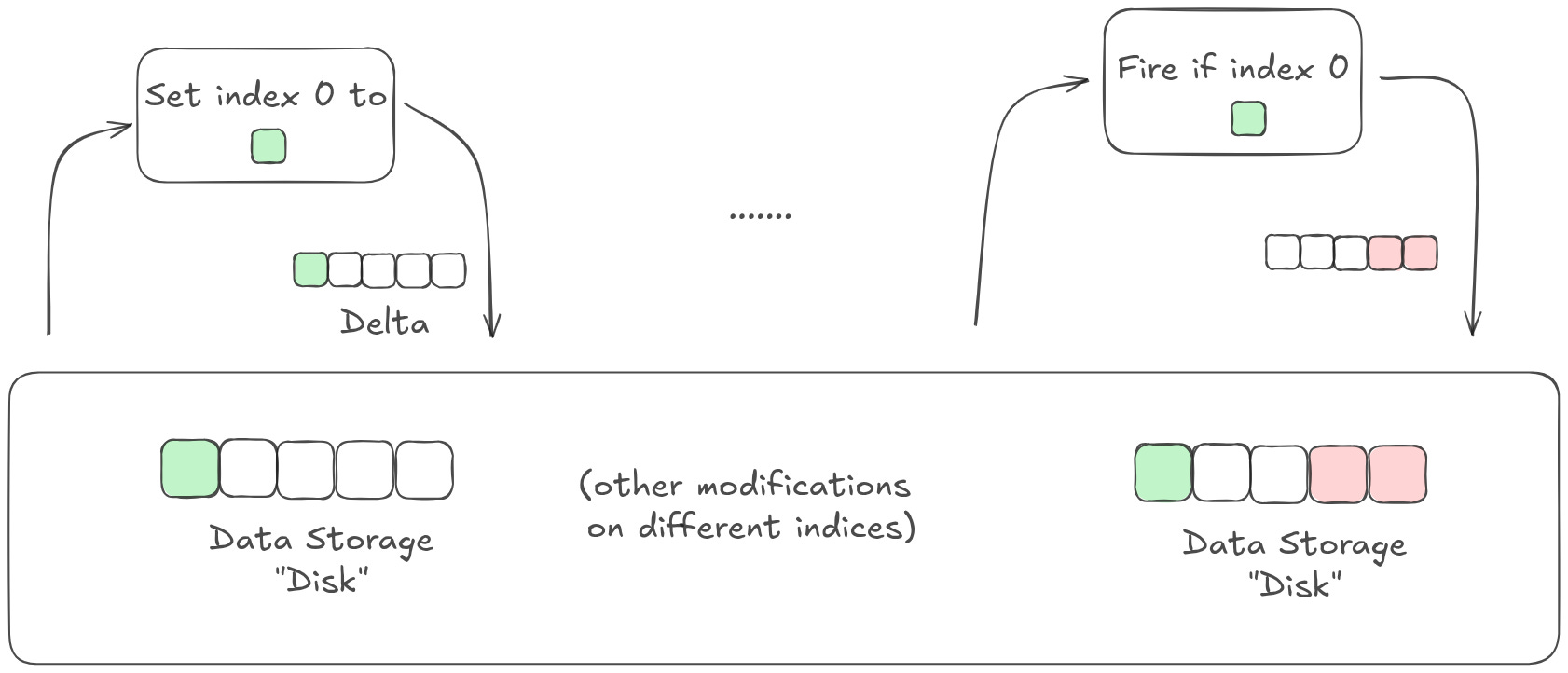
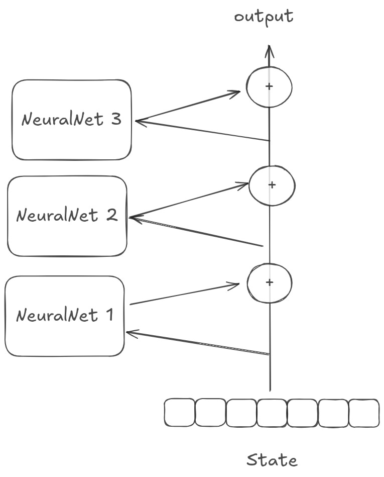
Identity residuals — commonly called a ‘residual stream’ — give a model a ‘scratch pad’ to use as state. Instead of learning how to transform a signal, each layer in a model learns a distinct ‘program’ that modifies the state. Importantly, layers don’t have to output any changes at all! A dimension in a residual stream will only change values if a layer explicitly ‘decides’ to change its value.
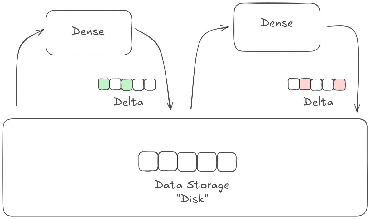
This gives the model a lot of flexibility. Much like in a traditional software system, different parts of the model can modify or even be triggered by other parts of the model; layers can communicate with each other even if they aren’t directly adjacent in the model stack, sort of like how different microservices can be called by each other as needed. In many cases, the state is set to some representation of the input. This means the model is, by default, learning how to modulate the signal that is present in the input data, instead of learning how to represent that data wholesale.
More generally, models with a residual stream behave fundamentally differently than models without one. The former distinguishes between programs and representations — you have a series of programs that determine how to update your representations, and a series of representations that are passed through. The latter is just program. You don’t really have representations that are independent of the stack of layers data is flowing through.
Operation: Learn multiple programs
Implementation: Convolution Filters, Attention Heads, Stacked and Parallel Weights
Certain kinds of models can really only learn one kind of operation per set of weights.
Take a convolutional layer — each filter in the layer is essentially fixed. Maybe it can learn an edge detector or a color change filter, but it can’t learn both. So to get around this, you stack a whole bunch of convolutional filters together.
More generally, we’ve discussed that you can create a “change in representation” with a matrix multiplication. If you squint, it’s possible that a model could learn some kind of conditional logic within that matrix multiplication. But in practice, that doesn’t actually happen. I think there’s a lot of reasons why (probably worth digging into in another post) but for now let’s take it as granted that a single set of weights learns a single comprehensive program.
To learn more complicated programs, you need to parallelize. You can parallelize “horizontally”.
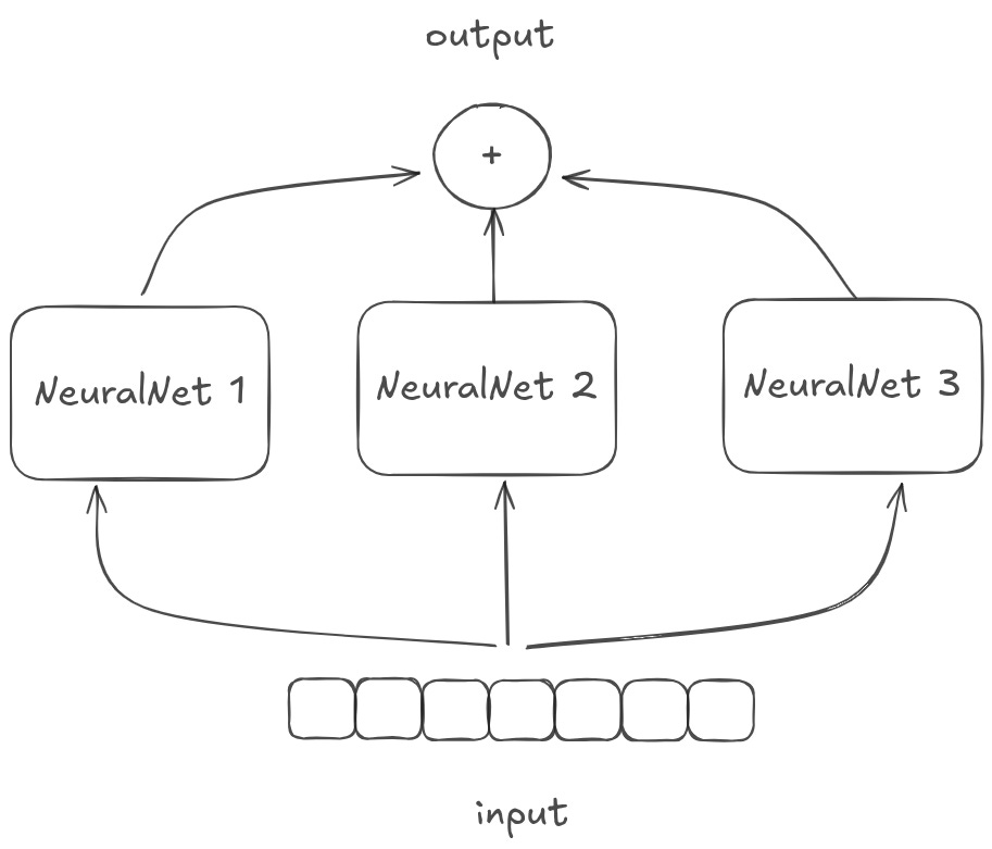
This is basically what multiple attention heads and multiple convolutional filters in a given transformer/convulational layer are doing. You should think of these as running multiple learned operations in parallel, and then combining the results.
Or you can stack vertically.
You should think of these as running multiple learned operations in sequence, each operation building on the last.
It’s not immediately clear what the benefit of depth is. We know it’s really good, but we don’t really know why. But one intuition is that stacking things vertically results in some exponential explosion of possible non-linear connections, and that in turn allows for more complicated programs.
Concluding Thoughts
This is all really fuzzy. There is no mathematical rigor here. I’m grasping at intuitions that I have, not formal proofs. Also, to make things worse, multiple operations are implemented the exact same way! How do you know when you are doing a weighted summary of a database or changing a representation of a vector? They are both vector * matrix matrix multiplications!
Still, as they say, all models are wrong but some models are useful. You can use the architectures above to predictably change how your models behave. So stay tuned for part 2, where we’ll walk through how some higher level operations can be broken down by the operations above.
Also, if you have other suggestions for operations that can be added to this index, let me know! There are probably other useful models and analogies that I’ve missed that can help demystify what neural networks actually do at an operations level.
Depending on the size of the GPT3 model, M ranges from 768 to ~12k.
Take a look at the Toy Models of Superposition paper for a really in depth look at how models represent and compress information.
Note that all distance measures can be inversely represented as similarity measures and vice versa, so they are used interchangeably here.
Approximately! Cosine similarity is scaled by the magnitudes of the input vectors, while vector x vector is just an unscaled dot product, i.e. the numerator of a cosine similarity calculation.
Note that no one actually does this anymore! In the Theano/Tensorflow days, this was basically the only way to do indexing efficiently on GPUs. But modern frameworks are better and more intuitive. Since a matrix is an array of arrays, the best way to look up a vector is to simply index into the first array to find the row that you want (see also: gather ops). But it’s important to understand how lookups work because it is the cornerstone of more complicated model architecture operations.
Side note: it’s reasonable to think that because you collapse the representations, you somehow tie the gradient representations to each other during training. In practice this is not the case. Application of the chain rule through back propagation results in each row having its own set of gradients, independent of the rest of the representations.