Ilya's 30 Papers to Carmack: Complextropy Redux

After reading this paper, I am beginning to see the sketches of an actual pseudo-quantifiable theory of model complexity.

This post is part of a series of paper reviews, covering the ~30 papers Ilya Sutskever sent to John Carmack to learn about AI. To see the rest of the reviews, go here.

Paper 20: Quantifying the Rise and Fall of Complexity in Closed Systems: The Coffee Automaton

Buckle in folks, this one is a ride. Also, note that this paper is directly related to, and is a formalization of, Paper 1: Complextropy.

High Level

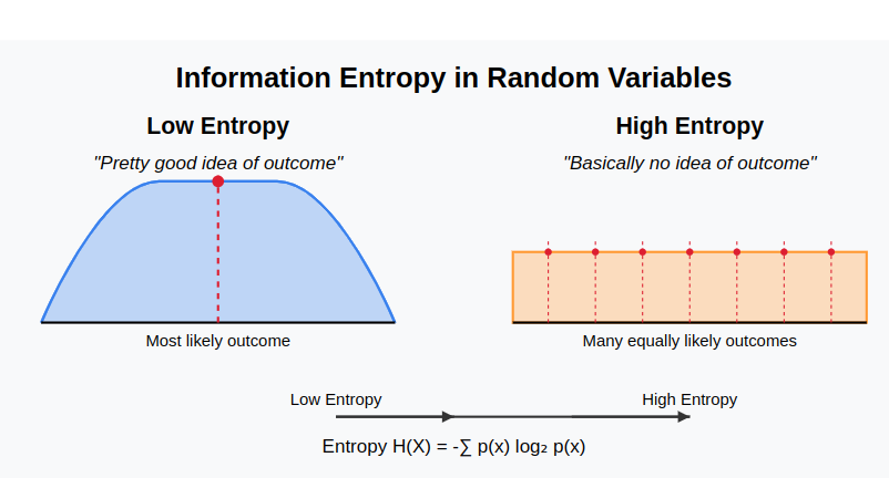
I never took any formal classes on information theory, and as a result I was always very confused about what this 'entropy' thing was. I knew, vaguely, that entropy was related to chaos. Physical systems 'trended towards entropy' which in turn is somehow related to disorder, or something. It wasn't until well after I left college, and indeed well after I left my research career at Google, that I decided to dig into this entropy thing and figure out what it was all about.

And, actually, it turns out the basic idea is quite simple. Entropy is a property of a random variable. In the same way a random variable has an expected value or a range, it has an associated entropy. Very roughly speaking, entropy measures the amount of information necessary to pinpoint a particular random variable state, given the entire spread. If you have a random variable where you have a pretty good idea what the outcome is, the variable has low entropy. And if you have a random variable where you have basically no idea what the outcome is, the variable has high entropy.

Entropy is a way to quantifiably compare the 'chaotic-ness' of random variables. It provides a mathematical language to explain why a coin flip is more certain than a dice roll, which is more certain than a slot machine.

In physical systems, entropy increases monotonically. All of the states a physical system could possibly be in is described by some random variable, and over time that random variable 'spreads out', the probable state space becomes more evenly distributed.

But entropy isn't everything.

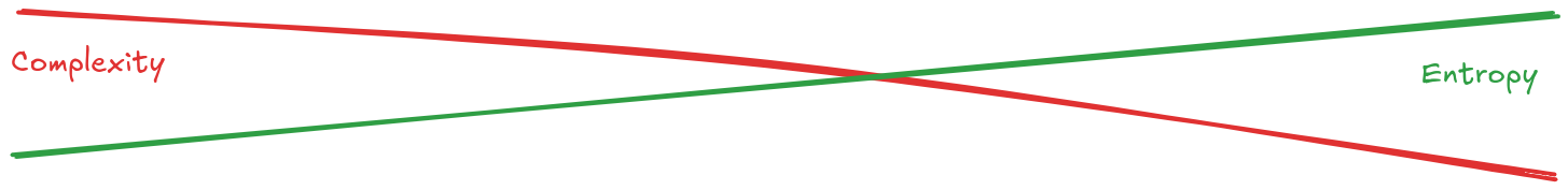
If you watch cream slowly mix into coffee, you may notice that the beginning state (low entropy) and the end state (high entropy) are actually somewhat similar in that they are both rather uninteresting. In the middle you get all these tendrils and interesting structures as the cream and coffee slowly merge together. On either end, you get a system that is pretty straightforward, and very easy to describe.

Or maybe if you think about the big-bang and the expansion of our universe. You start with this concentration of mass (low entropy) and end with vast nothingness as all the particles disperse into the void (high entropy). In the middle, you get galaxies and planets, solar systems and life. Again, on either end, you have this easy to describe system. But in the middle, all sorts of interesting things.

You could call this property 'complexity' or 'interestingness'. And what's interesting about 'interestingness' is that we do not have a good way to measure it.

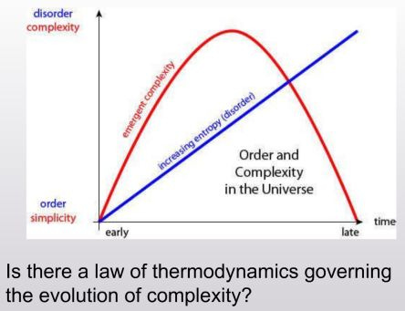
Is there some way in which we could compare the complexity of the universe to that of a cup of coffee? Can we create a quantifiable measure of how interesting something is? The authors of this paper aim to find out (spoiler: the answer is sort of).

The authors propose four ways to measure complexity as a distinct property from entropy. We'll go through the conceptual underpinnings of each in turn, though you'll have to check the paper for a more in depth treatment of the math.

Apparent Complexity

We have a pretty good grasp of entropy. We know how to calculate it — generally the entropy function is represented as H() — and we know how it increases in a system. One way to arrive at a good measure of complexity is to work backwards from entropy. Specifically, we want to find some sort of transformation f of a system x, where low entropy states are unchanged, and high entropy states are 'inverted' and represented as low entropy states. Symbolically, we could define this complexity measure as H(f(x)).

If entropy is a measure of noise, then you could think of f as a 'denoising' function. When the system has only a little noise, f will not do much. But when there is a lot of noise, f will do a lot. We can think of f as a method to remove 'incidental' information from the system. When the system is only incidental information, f will remove all of it, and the entropy of a system with no information left is 0.

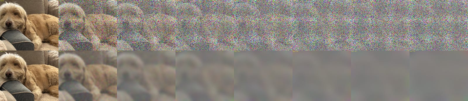
To make this all really concrete, imagine you had a NxN bitmap image. You could slowly add noise to the image, simulating increasing the entropy of the image. At each noise-addition step, the image will have some pixels that represent useful information, and other pixels that represent random information. You could get rid of the noisy pixels by using a blur effect. As the image gets more and more noisy, the blur effect will gray the whole thing out. Eventually, you're left with a gray blob — an image with no entropy.

On face this seems plausibly useful, but there's a tiny problem: we just, like, decided that our f function was going to be a blur effect. That's pretty arbitrary! As it turns out, f ends up depending on the type of modality, and possibly even the biases of the measurer— after all, how do you decide what information is important vs random? As far as measures go, this is a bit more suspect than entropy, which by contrast has a clearly defined formula regardless of where it shows up.¹

The authors argue that the choice of smoothing function actually isn't that arbitrary — they point to similar system transformations that are grounded in our physical observations:

when we observe configurations (whether with our eyes, or with telescopes or microscopes), large-scale features are more easily discerned than small-scale ones. (In field theory this feature is formalized by the renormalization group.) It therefore makes sense to smooth configurations over local regions in space.

Still. It would be nice if the complexity measure could just tell us what the distinction between random and non-random information is. So the authors plunge onward in their examination of other possible kinds of measures.

Sophistication

One other measure that is somewhat popular is known as Kolmogorov Complexity, generally represented as K. Kolmogorov Complexity is defined as "the length of the shortest computer program that outputs an n-bit string". So, for example, a string of n ones has a lower Kolmogorov Complexity than a random string, because I could represent the former as 1*n and I would have to represent the latter as the full string length.

Entropy is a measure of random variables, while Kolmogorov Complexity is a measure of a given object or state, e.g. a sample of a random variable. But Kolmogorov Complexity is closely related to entropy — intuitively, 111111 likely comes from a lower entropy random distribution than ajc13k. And, in fact, if you have a set of n-bit strings sampled from a distribution D, the Kolmogorov Complexity of any of those strings tends towards the entropy of D. Some of those strings will be more complex, some will be less, and they will hover around the average encoding length.

But unlike entropy, Kolmogorov Complexity is actually impossible to compute.² Sure, there are proxies — the file size of a gzip-compressed file is a decent approximation of K. But still, it's a weakness of the measure. Worse, Kolmogorov Complexity is also, counter intuitively, not actually a good measure of complexity as defined in the paper. We want our complexity measure to be low when there is only random information, and the Kolmogorov complexity of randomness is quite high!

Still, there's something here. Kolmogorov Complexity is all about having a principled way of understanding what information is important in a random variable. That was the big issue that we had with the previous complexity measure — in the apparent complexity setting, we were somewhat arbitrarily picking functions that would separate useful and not-useful data. Even if Kolmogorov Complexity itself isn't going to be a good measure of complexity, a derivative of Kolmogorov Complexity might point us in the right direction for a more principled complexity measure. The authors look at one such derivative, called sophistication (soph(x)).

The actual definition of soph is a bit convoluted. Imagine you had a set S of n-bit strings, and x is an n-bit string that is in S. We can say that the Kolmogorov Complexity K(S) is the length of the shortest program necessary to output S, and the Kolmogorov Complexity K(x|S) is the length of the shortest program necessary to output x, given that we know S. If you know S, then you can put an upper bound on the number of bits necessary to fully describe x within the set S — its log2(|S|), i.e. the number of bits necessary to uniquely encode every value in S. We may be able to describe x in a shorter way than log2(|S|). But if K(x|S) actually is about equal to log2(|S|), we are effectively saying that there is no more efficient way to compress x other than by identifying it as a part of S. Or, put another way, if S really captures all of the information that is worth knowing about x, then K(x|S) will be about the amount of bits necessary to just identify x in the set S. In this setting, the easiest way to represent x is to say that it is part of S, and, equivalently, S captures all the relevant or interesting information about x. This can be represented as a simple sum, K(S) + K(x|S) ~= K(x).

That was a mouthful. An example may help explain the concept. Let's say we had a string x = "11111". Already it's immediately obvious that this string has a lot of structure to it. But how do we define that structure? One way is to try and think about how you might explain this string. You could say x is a five letter string. That captures some of the relevant information. But there are a lot of five letter strings. "A5BgT" is a five letter string. We can get more specific by saying that x is a 5 letter string of numbers. This is much better, there are far fewer 5 letter strings of just numbers, but we still capture strings like 36235.

What if we said that x is a five letter string of repeating numbers? Now we're getting somewhere — there's only 10 of these, from "00000" to "99999". If we know that x is in this set, we can exactly identify x by simply defining it as the first index in this set. Here, all³ of the interesting information about x is captured by the definition of the set x is in, namely the set of 5 letter numeric strings where every letter repeats. The uninteresting information is just the position within that string.

As a reminder, Kolmogorov Complexity is the length of the smallest program necessary to output a variable. You can define Kolmogorov Complexity over a set too — in our example above, K(S) would be the length of the smallest program necessary to output the set of 5 letter repeating numeric strings, which might look something like: for i in range(10) print(i*5)

We've finally arrived at a definition of sophistication. Formally, soph(x) = min( K(S) ) for all S where K(S) + log2(|S|) <= K(x). In English, soph(x) is the minimum Kolmogorov complexity over a bunch of possible sets S that contain x, where the Kolmogorov Complexity of the set itself and the information necessary to describe x within that set is less than or equal to the information needed to describe x on its own.⁴ This splits x into two parts — a 'non-random' part specifying S, and a random part specifying x within S.

The upshot of all this is that we have a principled way of figuring out what is 'structure' and what is 'noise', and we no longer have to choose our own smoothing function. The function that maps x to S can be our smoothing function, and we have a principled reason for believing that is a good smoothing function.

Of course, we can't use any of this. What, you thought that I spent 1000 words explaining something useful? I told you at the beginning that soph(x) couldn't be computed! To calculate soph(x) you have to jointly optimize for finding S and all of the ways of encoding x within S. It's an ill posed problem.

Even worse, intuitively soph(x) remains low for most physical systems that we care about! Many systems can be described using a simple initial state and a simple probabilistic evolution rule. That means the overall state can be described with a very small program. We want a measure of complexity that rises and falls; even though in theory sophistication should display this behavior, in "practice" it mostly stays flat.

Other Methods

The authors discuss two other methods for thinking about complexity that are both eventually dismissed. To briefly summarize:

• Logical depth is similar to soph but it measures time to compute instead of length to compute. This works better for some strings that have small programs but have to run a long time to get them.⁵ But this measure also fails for the same reasons soph does — it's incomputable and a poor measurement in most systems we care about.

• Lightcone Complexity is a measurement of mutual information between the past states of an automaton and future states. If there is a lot of predictive power (i.e. the automaton is too simple), the lightcone complexity is low; and if there is no predictive power (i.e. there's no relationship) the lightcone complexity is also low. This is nice because there is a clear, calculable definition of this form of complexity. Unfortunately, you can't easily use lightcone complexity to describe past and future states of an automaton, since the complexity measure depends on those same states; there is no measure of 'inherent' complexity, only contingent ones. This makes lightcone complexity a poor measure across systems, which is sort of a key property of any good measure. It's also pretty easy to construct naive cases where lightcone complexity gives us the 'wrong' perception, because it is possible to have high mutual information between two states that are actually random.

As it turns out, all of these measures are somewhat related. I'm going to skip exactly why, feel free to take a look at the paper. But the long and short of it is, the authors end up going with apparent complexity as their measure of choice, largely because it is the only measure that is actually easily computable.

Experiments

At this point, the authors have arrived at a measure of complexity that they are kinda sorta happy with. There are some things that aren't great about it, but it's the best they could come up with. Now they want to test whether that measure is actually any good. Does their complexity measure actually correctly measure 'complexity'?

So the authors go back to coffee.

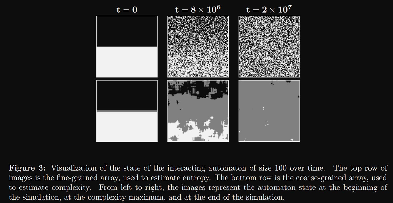
The authors create a cellular automaton simulation to describe 'coffee'. Each cell can either be 0 or 1. 0 represents coffee, 1 represents cream. The initial state is a square with all 0s in the bottom half and all 1s at the top half. The authors define two models, an 'interacting' model and a 'non-interacting' model. For the former, at each time-step, one pair of particle positions are swapped. For the latter, each 'cream' particle moves one step in a random direction, and the cream particles can all overlap.

The former model is more 'realistic', and as a result more complicated. There is no easy way to calculate or represent the various potential states of the model, short of indexing each possibility. The latter model is theoretically much easier to reason about — each particle is essentially just doing a random walk through the 'graph' of the coffee cup, so you can represent the model with a comparatively short program. As a result, the authors expect the 'interacting' model to show our desired complexity arc, while the 'non-interacting' will have low complexity throughout.

Applying apparent complexity to this numeric model isn't trivial. The authors need to define a smoothing function so that they can somehow capture important, useful structure from random noise.

Their first attempt to approximate apparent complexity is by using an algorithm called OSCR. OSCR works a bit like LLM Tokenization. Given a set of messages (in this case the total state space of the coffee automaton) OSCR attempts to find an encoding that minimizes the size of the "codebook" and the length of the "message". The great thing about OSCR is that it gives us a very principled way to identify 'useful' information vs 'noise'. In fact, the OSCR algorithm looks a lot like an approximation for soph — the "codebook" is equivalent to the set of strings S, while the "message" is the information used to identify a string x within S.

OSCR is essentially equivalent to Shannon Coding, which is grounded in information theory. It's also, surprise surprise, equivalent to optimizing for the Minimum Description Length (yep, the same MDL we discussed back in paper 6).

Unfortunately OSCR doesn't really work on this particular model — it doesn't compress the state of the automaton very well, possibly because the automaton is actually a 2D image and OSCR is designed for 1D string data.

So the authors fall back to thinking about kinds of coarse-graining algorithms, of which blurring is one. All coarse grain algorithms take in some 'microscopic' data and produce a 'macroscopic' representation. On images, you can course-grain using a straightforward convolution operation.

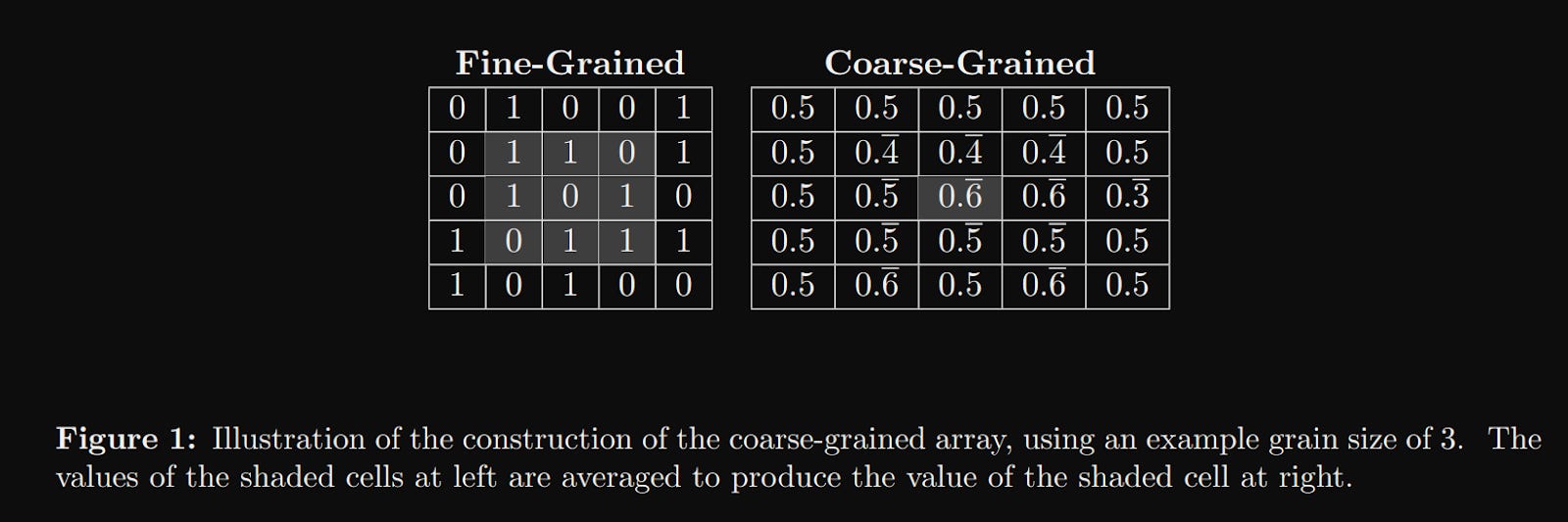
A convolution will take a really detailed image and produce a smoothed out one. Intuitively, we know that the smooth one has less complexity. But how much information is actually retained? The whole point of this paper is to try and calculate 'complexity' as a quantifiable measure.

Naively, we could approximate the amount of information in an image by looking at its file size. After all, in the detailed view, an image is nothing more than a width x height x channels matrix of numbers. But both our detailed image and our convolved "simple" image have the same shape, so they would have approximately the same file size. Still, the intuition is useful. I mentioned earlier that even though Kolmogorov Complexity is not easily computable, gzip and indeed any compression algorithm will act as a reasonable proxy. In the actual experiments, the authors run gzip to first compress both files, and then compare the delta of the compressed image sizes to get their complexity measure. Specifically, they treat the size of the compressed convolved image as K(S), the size of the compressed original image as K(x), and the amount of "random" information K(x|S) as the diff between the two K(x) - K(S).

Armed with a way to calculate their complexity measure of choice, the authors run the coffee automaton model and capture measures of both the entropy and complexity as the model runs. And they more or less get what they expected.

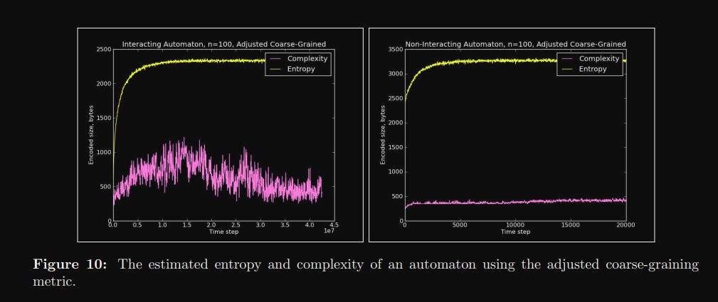
There's a bit more analysis on the behavior of these systems — in particular, the authors discuss different adjustments to their coarse-graining strategy, as well as various measures of maximum complexity and how that changes with the model size — but I'll leave off here. We got to the interesting meat of the paper, and my brain hurts.

Insights

Before we talk about the ML side of this, I just want to comment about how interesting and weird this paper is to me. It frankly never occurred to me that one could write a paper on a subject like "coming up with a way to quantifiably measure a concept". Maybe there's some discipline where this sort of work is very common (I guess this is maybe measure-theory-ish?) but none that I've ever read before. At first, I hated this paper, because I just couldn't understand why it mattered. Like, yes, great, you came up with a measure of complexity that you made up yourself, and then basically worked backwards to find an experiment that showed exactly what you wanted, and even adjusted the experiment a bunch when it didn't quite show what you wanted the first time. This is the reverse of the scientific method, but whatever, big whoop-de-doo.

I think I really did not get this paper the first time I read it, and really arguably the first three times I read it, because as mentioned this paper is a formalization of the very first paper we reviewed. But on a fourth read through, I think I finally got it. I also found a really deep appreciation for what the authors — and in particular Scott Aaronson — are trying to do. They set out to find a principled way to measure an observable, seemingly universal phenomenon. It's clear that they are looking for something that is elegant and generalizable, akin to entropy, and in that effort they did not quite succeed. But this is a monumental undertaking, and if they had found something workable it would have potentially revolutionized our understanding of physics AND mathematics AND information theory, in the same way entropy did. After all, they are essentially hunting for a yet-undiscovered property of physical systems in general.

And even though they did not exactly figure out a good definition of complexity, it is immediately clear that complexity shows up all over deep learning, on many different levels.

When we first encountered this concept all the way back in November, I wrote:

There’s something intuitive about the idea that systems become more complex before they become less complex, even as they gain entropy. I think this is because the ‘manifold’ of entropy has a bunch of minima and maxima. In other words, as you gain entropy, you may end up creating some structures that are higher entropy than the baseline condition, but still lower entropy than the highest possible entropy state. I feel like I’ve seen similar properties outside of coffee cups, especially in biology — this paper reminded me of enzymes acting as a catalyst to make some process occur. You need the enzyme (structure) to go from a low entropy state to a high entropy state (pre to post chemical reaction).

My recent new favorite paper is Toy Models of Superposition by Anthropic. It is a BEAR of a paper. Really long. But take a look at this figure:

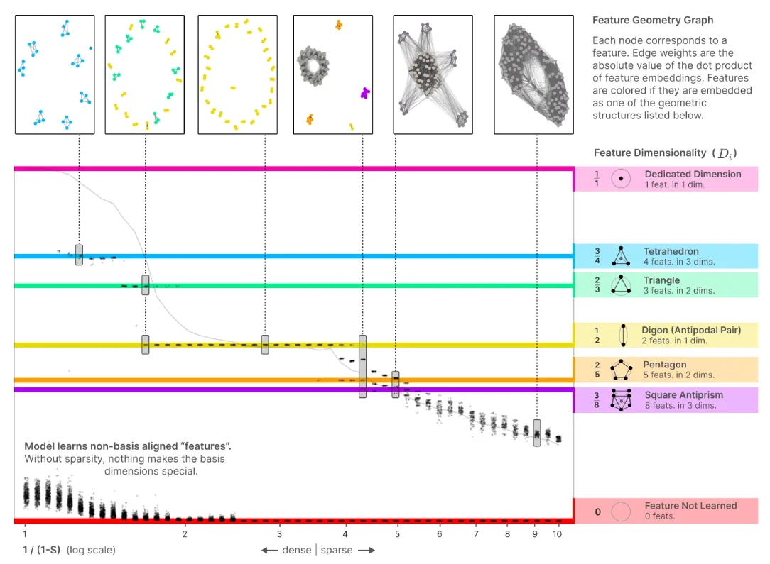
This figure shows that as a model tries to represent more and more features, it begins to take on complex structure in its underlying embedding space. It starts without any structure, and ends with every feature touching every other feature. Both of these are not very complex. And then in the middle you get all of these weird patterns — tetrahedrons and triangles and digons and square antiprisms. Sounds pretty complex to me!

So already there's a nuts-and-bolts way in which the model's internals are explicitly modelling this complexity 'arc' structure during training — if you were to map the apparent complexity or sophistication of the model internals over time, you would get a nice parabola as a function of entropy.

After reading this paper, I’ve also come to appreciate just how much complexity is interwoven into ML theory. If you take a big step back, neural networks and other forms of ML models are all methods of representing some dataset X. Not all datasets are created equally. Some are really simple and easy to model — for example, MNIST. And others are really complicated — for example, the entire internet. Intuitively, we know that MNIST is easy for neural networks to learn. A simple multi-layer perceptron does a decent job. And we also know that the internet is quite difficult for neural networks to learn. You have to train a massive multi-stage transformer model with billions of parameters.

One reasonable question to ask is whether there is a way to quantifiably compare how complicated different datasets are. Well, from this paper, we know that every dataset can be split into ‘important’ information and ‘unimportant’ information. The former somehow captures the ‘important structure’, while the latter is noise. Also from this paper, we know we can represent that important information as a set S that contains all of the samples in the dataset, as well as other related data that may not be directly in the dataset but has the same structural properties. And we can represent the unimportant information as the index of a particular data point is the larger set, x|S,

Hopefully the application to deep learning is clear. We want our models to learn S. That is, we want our models to capture all of the interesting information about the random variable(s) that represents the training set. But we don't want our models to learn the random noise that allows us to identify random particular elements within the training set. A given sample of the training set x should be represented by the model weights S plus some additional information conveyed by the input data sample, x|S. If S ends up being too precise, it will not generalize well to data points that are not in the training set, because those data points will not be in the underlying set the model is representing!

But wait, how do we ensure that our model is not too precise? Well, going back to our discussion about soph, it is not enough to just get any set of data S. In order to actually calculate the complexity of a dataset soph(x), we have to find the set S that has the minimum Kolmogorov Complexity K(S) among all of the possible sets that also represent x efficiently.

This is just Minimum Description Length theory!

Pulling from my review of the MDL paper:

Minimum Description Length theory (Sections 1 - 4), roughly states that the “optimal” model to represent a set of data is “the one that minimizes the combined cost of describing the model and describing the mis-fit between the model and the data” — that is to say, it minimizes training loss AND model size. Why might the MDL be true? Imagine we only cared about getting a really low loss on our training data — for any model that generates some loss, we could always make a bigger or more complex model which would generate a smaller loss. But of course, doing so makes the model worse at predicting new data (because of overfitting, above). “So we need some way of deciding when extra complexity in the model is not worth the improvement in the data-fit.” Thus, MDL.

Originally, I assumed that this was just true simply because of empirics — that is, when you let the model overfit it does worse, so obviously you want to penalize the model, and look it does better when you do that. But after reading this paper, it’s clear that the basic theoretical principle behind MDL derives from our discussion of Kolmogorov Complexity and soph in this paper. In the MDL paper, Hinton says that the optimal model minimizes the cost of describing the model and the misfit from the training data. That is, we want to minimize K(S) + K(x|S) for all x in the training set. Look familiar? This is basically just the optimal soph measure! The minimum value of those terms is when we find a set S that captures all of the useful information.

In this framing, model training is nothing more than finding the right set S. The model starts by representing some set that is too broad — it takes a lot of additional information to correctly identify the training sample within the set. We need the model to narrow down the set it represents. But if we only optimize training loss, the model will never narrow S because it does not need to. So, in turn, we need some way to capture the size of the model K(S) in our loss function. As per Hinton, we can do this with regularization terms in the loss. With these additional terms, the model will narrow the set it represents until the amount of additional information needed to identify the training samples is small. This is essentially a theoretical way of saying that neural networks are compressed databases. When trained with regularization, the size of a neural network and its loss is a way to accurately measure the complexity of a dataset.

Maybe all of these parallels were obvious, but all of this is a very new way of thinking about neural networks for me. The ability to link model learning with Kolmogorov Complexity explicitly is really interesting, and it gives a lot of handholds on thinking about AI models. I've been thinking about how to fit model architecture within the wider lens of information theory, so I'm hoping to come back to this particular thread.

One last thought.

Earlier, I mentioned that a big problem with the Apparent Complexity measure is that you have to define some smoothing function f to help remove noisy information, and unfortunately there is no principled way to identify which information is 'important' and which information is not. As it turns out, there is a sense in which neural networks themselves are a principled way of compressing information. You can think of the neural network as learning the smoothing function f implicitly in its weights. A well trained model will carry within its internal representations all of the important information. And we know f is principled, because it is defined by optimizing (minimizing) the amount of information required to compress a training set.

This immediately made me think of VLAEs and Diffusion models.

VLAEs explicitly learn a high-level embedding space without any 'noisy' fine grained data. The VAE embedding smooths over detailed information that is captured by an RNN during training, providing exactly the same dichotomy of 'important structured information' and 'unnecessary noisy information'. Pulling a figure from my review of that paper:

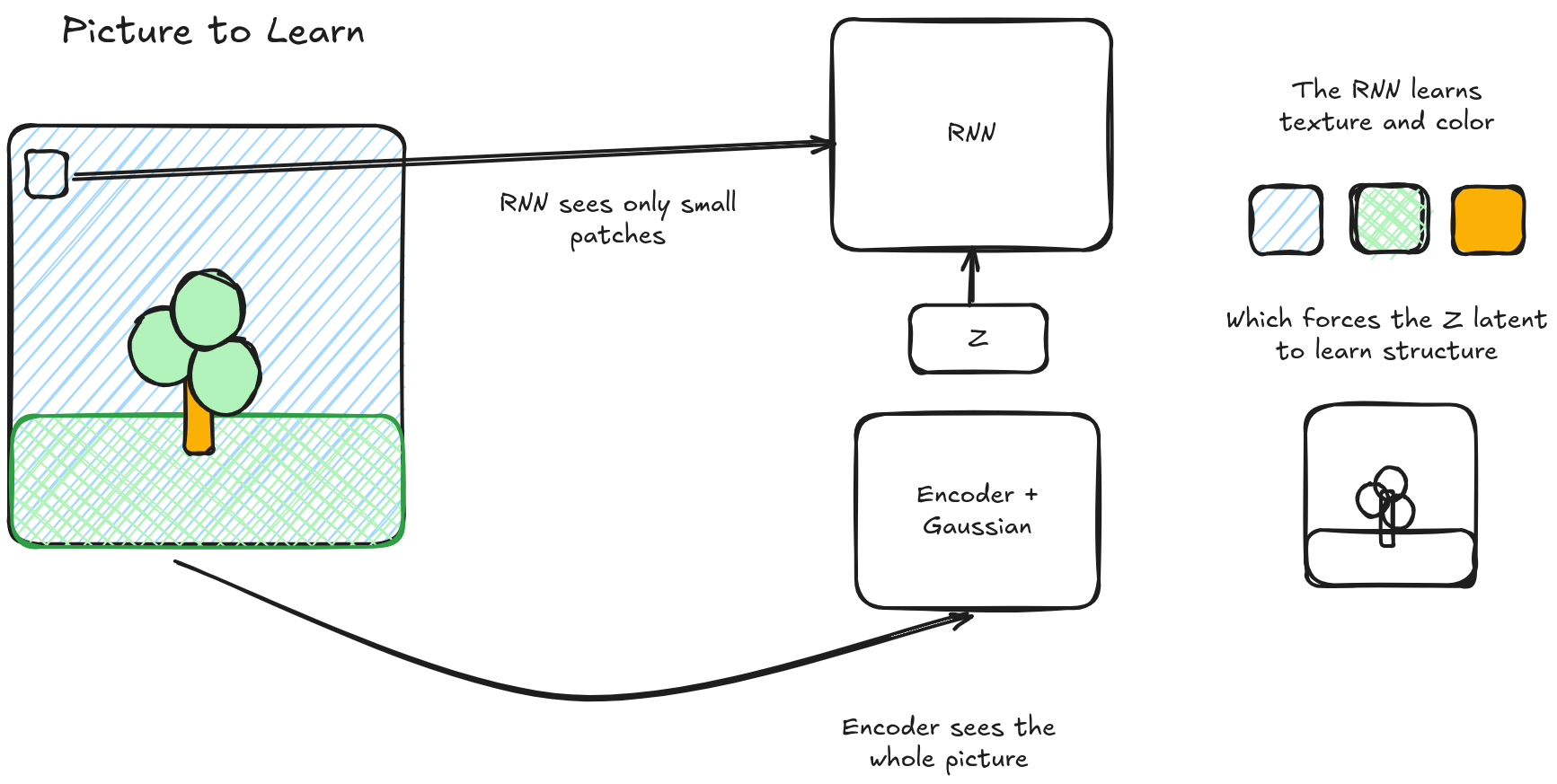
If a normal neural network implicitly learns a smoothing function f, VLAEs are all about making that smoothing function explicit. In a VLAE, the RNN acts as an inverse of the smoothing function f described in this paper — in the inference pass, the RNN learns how to add granular information that is missing in the underlying latent. As a result, the latent does not need to learn anything about that particular set of information. And since that information isn’t needed, it is smoothed out of the embedding space as a natural consequence of the model optimizing to represent other things. So the VLAE gives us a way to directly control what smoothing function the model learns.

Diffusion models take this all a step further and are even more directly ‘principled’. A standard diffusion model learns to reverse entropy from some distribution. In images, they start with some noisy input and successively learn to remove that noise. So, implicitly, the diffusion model is somehow distinguishing between noise and structure. Unfortunately, with diffusion models, that distinction is totally implicit. With a VLAE you can extract the latent encoded z space after the model is done training; no such easily extractable latent exists with diffusion models. There’s more that can be said here, but to do that we’d have to dive into how diffusion models work in detail. I’ve recently been reading a lot of diffusion papers and I’m hoping to do a more full pass on diffusion soon, so I’ll leave off here.

---

Oof. Very long paper. Thanks for sticking around to read the whole thing!

1. In fact, it's a bit of a meme how many things basically just end up being some variation of entropy.

2. Trying to find the actual Kolmogorov complexity of a random variable is akin to solving the halting problem. See wiki for more.

3. Sort of. Remember that this is actually impossible to calculate. So we can't explicitly say all, because there might be a better formulation of the set that captures more information about x.

4. We use a minimum because there are many possible sets S that may fulfill the given condition.

5. The authors didn't really provide an example of this, and I didn't spend a ton of time thinking of one, since it's not super relevant to the paper