


Ilya's 30 Papers to Carmack: VLAEs

This post is part of a series of paper reviews, covering the ~30 papers Ilya Sutskever sent to John Carmack to learn about AI. To see the rest of the reviews, go here.
Paper 18: Variational Lossy Autoencoder
High Level
Machine learning practitioners tend to be a bit handwavy about their terminology. In part I suspect this is because we don't really know what we are talking about most of the time. As a result, many terms converge and others take on colloquial meanings that maybe aren't fully correct.
I definitely am not as precise with my language as I should be — I often will say that 'representation learning is key to understanding deep neural networks' and will talk about embedding spaces as if all models are learning some sort of principled representation. There is some truth that all models are learning some kind of "representation", where they are turning information into vectors and back again. But there is no guarantee that the space of vectors is well formed. If we are learning a car classifier, we want it to be the case that the school buses are close to the trucks and far from the motorcycles. Since we only have a limited amount of data, though, the model may end up learning a classifier that has the buses next to Ferraris, or whatever. Often, the specific choice of model determines the quality and structure of the vector space.

Another word that is often used imprecisely is the concept of a 'latent' variable. A lot of folks use 'latent' to simply refer to 'the intermediate layers of the model'. So latent variables, embeddings, vector representations — in the common terminology, these terms have all sort of bled together. But a latent variable has a specific meaning: it is a variable that represents some kind of compressed representation space. Not all embeddings are necessarily latent variables. And in this paper, we are specifically interested in probabilistic latent variables. These are vectors that are produced by some probabilistic generator, commonly a Gaussian function, which is used downstream to calculate the output. And often the model is feeding parameters into the probabilistic function — for example, the model may calculate and pass in a mean and standard deviation, and then get out a vector variable sampled from a Gaussian with those parameters.
It's reasonable to ask why you'd want to feed in seemingly random noise. Surely that would just degrade the model performance? One intuition is that the gaussian generator smooths out your vector space. A model without any probabilistic latents will eventually learn to overfit to the data it sees, creating regions of the vector space without any 'density' that are essentially just noise. The probabilistic latent variable prevents that — a given input no longer represents a single point, but rather is mapped to a smooth area. In addition to being a form of regularization (see MDL review), the hope is that by inserting one or more random structured variables, the model will have some scaffolding to structure the high dimensional representation space around. That in turn may result in a representation space that is 'well formed' — the buses are near the trucks and the ferraris are near the lambos and the motorcycles are near the mopeds and all of these things smoothly transition between each other.
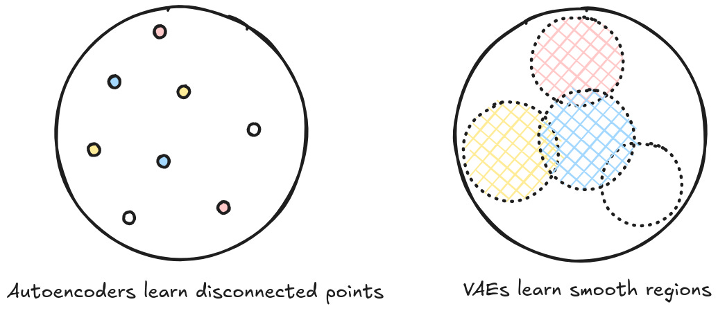
Because latent variables learn a 'space' of representations, they can be used to sample more data than what is provided from the training set. Models that have this behavior are called generative models because they are explicitly modeling a distribution. That is, instead of learning some classification (what is the likelihood that this picture is a cat given an image with a specific arrangement of pixels, p(y | x) ), they learn how all of the relevant variables interact (how often does this particular arrangement of pixels correspond with the label cat, p(x, y) ).1
This brings us to the paper.
The authors pose a problem. They want to create representation spaces that can disentangle things that are 'useful', but normal models often just learn to overfit on garbage noise. For example, we may want to create a model that is good at representing images. Naively we want the images that have the same 'global structure' to be next to each other — outdoor scenes near other outdoor scenes, urban cityscapes near other cityscapes, etc. — but the model ends up splitting images based on something unintended like brush stroke patterns.
It's sort of obvious why this happens. We aren't showing the model the 'true data distribution', we are just showing it a small set of samples. There are a lot of different functions that can output the same observed data distribution. To get to one that also encodes reasonable structure, you have to condition the model somehow. Still, this makes 'generative modeling' ill-posed — you have to define what a "good" model means first!
Normally, AI practitioners use models like variational autoencoders (VAEs) to do representation learning, because they naturally have a clear hierarchy of latent variables. But there are other models, like RNNs, that are really good at generative modeling (e.g. autoregressive text generation) even though they don't have latents at all. Since representation learning of this form is naturally a generative task, this raises the question: can you combine an RNN and a VAE?
Surprisingly, the answer is no! At least, not trivially.
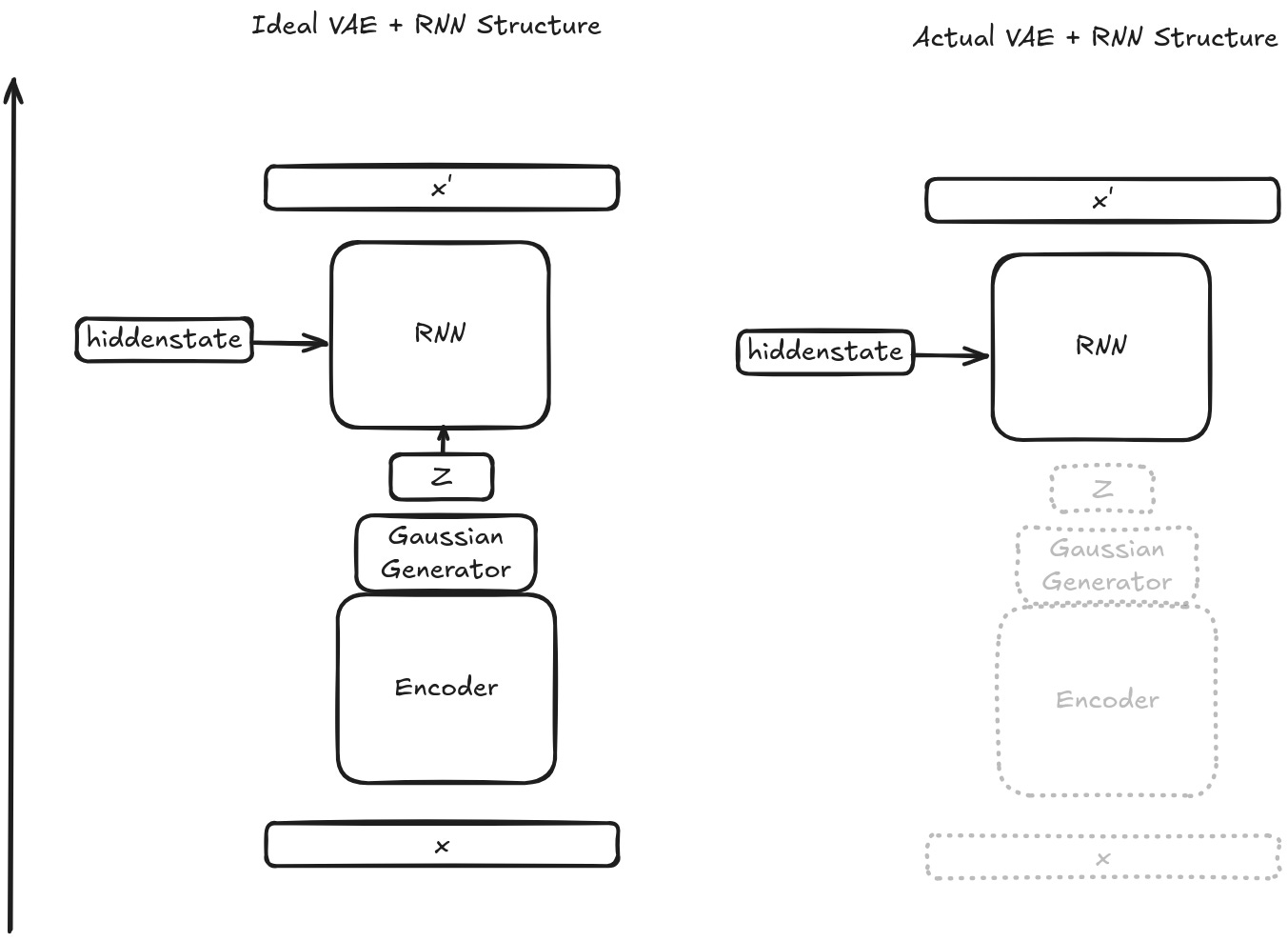
Like all auto encoders, a VAE has an encoder and a decoder. In theory, you could stick an RNN in the decoder slot. At each step, the RNN would take in all of its previous outputs and the latent encoded vector from the VAE to output the next word/character/token in an autoregressive way. Intuitively, if you train this system right, you can put all sorts of interesting global structure in the VAE latent. Maybe you want the RNN to output things that are "happy" or "sad" or "formal" or "informal", or maybe you want it to have the ability to reference back to some important context that might otherwise get lost over long generation sequences. If the RNN learns to condition on the VAE latent, you could plausibly do all that and more just by tweaking the latent variable at inference time.
In practice, previous papers have shown that if you just naively stick an RNN as the decoder of a VAE, the RNN part overpowers everything. Specifically, the RNN is able to represent everything it needs without relying on the structure of the latent variable, so the model learns to just set the weights that ingest the latent to 0 and ignores it entirely.
The author's propose a pretty straightforward solution, but I want to go on a tangent first. To really understand what the authors are doing, we need a better understanding of what a VAE actually is, and how this all relates to Maximum LIkelihood Estimation (MLE). If that's not interesting to you, feel free to jump a few paragraphs (cntrl-f "back to the paper").2
Let's say we have a scatter plot with data that is sampled from some distribution, X = { (x1, y1), (x2, y2)... }. We want to learn a generative model that tries to predict the original distribution the data was sampled from. Note how this differs from standard classification. We are not trying to figure out y given x or anything like that. We are trying to directly model the real original data source, with all of the variance between x and y baked in.
We can represent our model with a set of parameters, θ. We want to find θ that best 'explains' the data that we see. In other words, we want p( X | θ ) to be high. This is called 'maximum likelihood estimation' — we are finding the model that has the "maximum likelihood" of producing the observations we see.3
This is an intractable problem, even in the simple 2d case. The true distribution of data could be something simple like a Gaussian, or something arbitrarily complicated.

The number of parameters you need in your model is directly dependent on the shape of the true distribution. But you don't know the true distribution of the data! So you have to look at the data and guess what the shape might be. This is called a 'prior'. One simple example of a 'prior' is "I assume my data was sampled from a line". If you assume the data is a line, you have two parameters θ = { m, b }, where m is the slope of the line and b is the bias.
MLE requires you to sum the 'likelihoods' of each observed data point, given a particular model. One way to do this is to trial and error a bunch of lines and see how well they 'fit' the data. Or, put another way, we propose a model, calculate the 'likelihoods' of each data point given that model, and then sum them all up to compare across models and choose the best one. I'll shortcut to the end: for 2D linear data, this is how you derive least squares linear regression.
2D linear data is pretty straightforward, and actually has a closed form solution that can be derived by calculating the derivative of the least squares equation, setting the value to 0, and then solving for θ. But things get harder if you are dealing with high dimensional latents. And if your model has a probabilistic latent variable in it, you need to integrate over that latent in order to figure out the probability of producing any given data point. This is essentially computationally impossible.
So we can't directly optimize for the MLE for generative deep neural networks.
One alternative is to optimize the variational lower bound instead of the MLE. First, you introduce a stage in your model that produces parameters for a probabilistic latent variable — quoting from above, "the model can calculate and pass in a mean and standard deviation, and then get out a vector variable sampled from a Gaussian with those parameters." And then you treat this whole thing as an auto-encoder loss. You have a model that is learning q(z | x) — the 'encoder' that produces some latent variable from this probabilistic generator. And you have a model that is learning p(x | z) — the 'decoder' that turns the latent variable back into the original input. Train that all jointly, and you have a 'variational autoencoder'. Which is basically just a complicated way of saying 'an autoencoder with a random variable smoothing out the bottleneck layer'.
Ok, so back to the paper.
Jumping out of math/theory world, if we think about model architectures it should be immediately obvious that the encoder and decoder can be any kind of structure. You can have an RNN or LSTM for the decoder, and a conv net or mlp for encoder, or vice versa. And all of these can be trained jointly with backpropagation flowing end to end. In an ideal hypothetical, both the encoder and decoder are already trained, which in turn means the latent variable z (the output of the encoder) carries a lot of relevant information about the input data point that the decoder can actually condition on. But in practice, at the very start of training, everything is random! There's no information stored in the latent at all! And so what researchers find is that if you have an 'expressive' decoder like an RNN, it just learns to ignore the latent entirely.
It gets worse. Even if you manage to solve the training optimization issues, the authors show that it's always optimal for the RNN to ignore the latent variable. This goes all the way back to the Minimum Description Length (MDL) paper. Quoting from that review:
…the “optimal” model to represent a set of data is “the one that minimizes the combined cost of describing the model and describing the mis-fit between the model and the data” — that is to say, it minimizes training loss AND model size. Why might the MDL be true? Imagine we only cared about getting a really low loss on our training data — for any model that generates some loss, we could always make a bigger or more complex model which would generate a smaller loss. But of course, doing so makes the model worse at predicting new data (because of overfitting, above). “So we need some way of deciding when extra complexity in the model is not worth the improvement in the data-fit.” Thus, MDL.
Earlier we said that the probabilistic latent acts as a form of smoothing or regularization. We use regularization to bake in the MDL principle in the model's loss function — with regularization, the model is more likely to try to minimize its description length and therefore avoid overfitting. And intuitively, it's strictly less efficient to represent a data distribution with an RNN and a latent variable than with an RNN alone. So the model will basically always ignore the latent variable entirely.4
In slightly more technical terms, VAEs are trained using an ELBO loss (not going to get too deep into that here, but here's what wikipedia has to say). It turns out that optimizing for ELBO is also equivalent to optimizing for model complexity. So we can reframe the use of the latent space: the model will only use z as a probabilistic latent if doing so is more efficient than representing the input distribution directly. If z is at all different from x you end up with a regularization term in your loss — the KL Divergence of the two. With a strong enough decoder, the model can basically always artificially set the KL Divergence term to 0 by bypassing the latents entirely. An RNN is such a decoder — it can learn to bypass the latents by relying entirely on its own hidden state. The RNN learns the entire data distribution directly and passes it from step to step, so it never needs to rely on the z to do anything. Oops!
Hopefully by now we have a deep understanding of what the problem is. Can we leverage that understanding to get our models to do interesting things with the latent variables even when using autoregressive RNNs?
The authors notice that any information passed to the RNN will never appear in the z latent. So they decide to cherry pick what information the RNN can see, and assume that the "rest" of the information will have to be encoded in the z latent.
For example, imagine you were trying to learn to predict the ‘next’ pixel in an image given all the previous ones. You want your z latents to learn global structure, but not texture. One way to force the model to rely on the z latents is to give the decoder information that we don’t want in the z latents — in the example provided, you could represent texture through a small window around the pixel. During training the model will never utilize the z latents to store texture information, because it already has an easier way to access that data directly. But it will be forced to use the z latents for the larger global information, because the decoder itself is limited to only looking at the last few pixels while the z latent has the whole thing. Here, we handicap the RNN to prevent ‘posterior collapse’ of the z latent, while simultaneously encouraging the model to pack specific kinds of information into the latent.
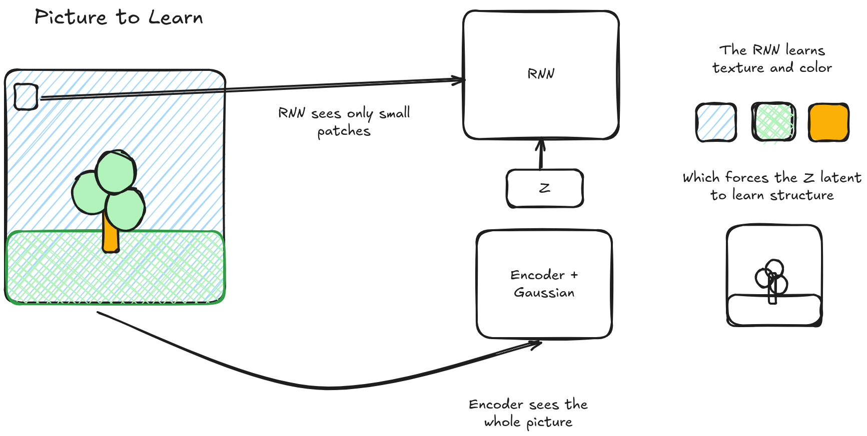
And of course, you could do the opposite — you could show the model a very low resolution image each step, forcing the encoder to pack in local ‘high resolution granular’ data into the latents.
The authors call this a variational lossy autoencoder, a VLAE — lossy because the autoencoder part isn't learning the complete information, as some of it is being carried by the RNN hidden state.
The authors modify the VLAE a bit more by using an 'invertible autoregressive flow' on top of the Gaussian to produce their final z latent variable. You can think of an IAF as a series of neural network layers on top of the Gaussian. Unlike a standard fully connected layer, the IAF is 'auto regressive' — each dimension of the output is a function of a sequential subset of the input.

Because IAFs are more expressive than a standard gaussian output, the theory is that z has less of an impact on the KL divergence regularization term, which in turn results in the latent being used more.5
Since the VLAE is purposely learning a lossy representation, the authors are interested in learning just how lossy it is. So the experiments are all about how well they can reconstruct some underlying image representation while having a more compressed representation. I'm not going to dive too deep into those here, except to say that it's definitely interesting to see what the model ends up encoding in latents and what it chooses to avoid. For example, the authors note that some of the image reconstructions end up losing color information, likely because color is very easy to predict from local information alone, so the color data never makes it into the encoded latent representation.
Insights
As I've read through this list of 30-ish papers, I've started categorizing different papers into threads. One paper might propose an idea and a different paper might pick it up a few years later, following a similar theme. These threads are rich conversations, with folks responding to and building upon each other's ideas.
One thread is what I've been calling the "complexity" thread. This thread is all about model complexity — how can we measure it, how does it behave, when do we want more or less complex models, things like that. And we've already seen a few papers in this thread. The MDL paper was the first chronologically, which laid out the idea that model complexity is something we actually should care about minimizing. And the complextropy paper followed up by trying to define a measure of complexity that we can actually reason about.6
VLAE builds on these concepts of complexity by using them to justify and guide a particular model architecture. In particular, we can use our understanding about how regularization modifies model complexity to explain an otherwise confusing and unintuitive result — that RNNs don't use latent encoded data. This is pretty cool!
The VLAE paper is also a representation learning paper. In fact, it's really the most representation-learning-paper we've hit thus far. We've talked a bit about representation learning in the review of the MPNN paper and the original attention paper. In those settings, models are learning implicit representations of concepts but aren't really learning representation spaces. The VLAE is explicitly architected to learn a latent space. You can adjust the latents in a smooth continuous way and get representations that 'make sense' along the vectors you choose to move in.

This is partially why the authors are so interested in understanding just how much they are able to compress their representations. Almost all interesting representation schemes are lossy, the question is always 'how much' and 'along what axis'. Most generic compression schemes (think: jpeg) are semantically indiscriminate. You cannot tell a jpeg to 'care more' about the structure of a house vs the color of the sky, for example. If the authors can use VLAEs to consistently regenerate the information they care about using a very small vector representation, they have created a very powerful semantically aware compression algorithm. This was always the promise of auto-encoders in general, so it's cool to see how that particular area developed.
I think this paper is also just a fascinating look into how models learn. There's some deep intuition to be gained here — if you can grok why the RNN will always ignore the latent variable, you've understood something fundamental about how models learn things that is difficult to put into words. So much of deep learning practice is about these intuitions. How does information flow? Where is it stored? How do different training regimes and architectures change information representations? And so on.
All that said, looking back from 2025, I think we've mostly as a field moved away from using probabilistic latents in popular benchmark-breaking models. There are some areas of research like the Bayesformer, but most representation models these days use some form of semi-supervised loss like CLIP (contrastive loss) or BERT (self-token-prediction). These methods scale much better with massive data repositories, which seems to be more useful than inlining smoothing functions using embedded random variables.
Note that there is a bit of a blurred line between learning conditions and learning joint distributions. You can train a classifier to learn conditions, but then simply take an intermediate embedding representation from that classifier and use that to generate new data. The intermediate representation may not be very good, but it is possible, and that makes this whole conversation a bit fuzzy — like everything else in deep learning.
In deep models, MLE provides a theoretical grounding for figuring out your loss function. Cross entropy loss or MSE are instantiations of maximum likelihood estimation given certain priors, like categorical data or a gaussian distribution, respectively. That said, in practice I think you can mostly ignore MLE and just short-hand it to ‘cross entropy loss for categories, error losses for regression’.
This was always hard for me to understand because it felt backwards! I always thought you would want to find the parameters conditioned on the data points. But the data comes out of the model, not the other way around.
That's not to say that MDL is wrong. MDL refers to the complexity of the model and the number of bits necessary to communicate the data through the model. Latent variables introduce a form of a loss term on the model complexity but don't capture the total complexity. The theory behind a RNN + VAE is that the combination may be a more complex model, but should significantly reduce the total complexity by decreasing how difficult it is to represent data.
I'm not fully clear on why they needed this to be an IAF instead of a standard mlp. The IAF does have some additional structure, so maybe that helps in some way?
Spoiler: the coffee automaton paper that is coming up in Paper 20 is also in this thread.