This post is part of a series of paper reviews, covering the ~30 papers Ilya Sutskever sent to John Carmack to learn about AI. To see the rest of the reviews, go here.
Paper 13: Neural Message Passing for Quantum Chemistry
High Level
The MPNN paper is interesting because it's simultaneously a survey paper, a modelling paper, and an applied-ml paper. There's a lot of rabbit holes that we can dive into here, so I'm going to break things up into subsections to try and make things flow a bit better.
The MPNN paper is framed around a problem space: can we predict certain properties of molecules from their structure alone? There's a lot of reason to believe we can — molecular structure directly determines all downstream properties in a chemical/physics sense. But this is also a hard problem to directly solve for. In 2017, we don't even understand what structure is even created for a given molecular sequence, much less how structure leads to function1.
But maybe we don't need to. Maybe we can just throw enough sequences and their corresponding properties into a neural network and have the network learn, in some fuzzy way, what the structure does.
One challenge with doing this is that molecules are best represented as graphs. A graph is a structure with an inconsistent number of nodes, each with an inconsistent number of edges. Graphs are really expressive and appear all over the place. Social networks, transaction networks, road ways, disease spread — all of this and more can be represented using graphs. But that same flexibility makes it hard to represent in a way that a neural network can ingest. Neural networks are stacks of matrix multiplications. And matrix multiplications require fixed-sized dimensions along some axis to work. Put another way, you instantiate and train a neural network with a fixed number of weights, which in turn represents a fixed amount of computational capacity. How does that work with graphs that are fundamentally variable?
MPNN Framework
The MPNN authors look over a wide range of papers attempting to solve this problem and come up with a generalized "message passing" formulation:
In English, this equation basically assumes that every node and every edge has some vector representation associated with it (h and e respectively). And then it defines two functions:
a "message passing" function, M by which a node "collects" information from all of its neighbors to construct a 'message';
an "update function", U, that applies the message to update the node's own representation.
A few things to note about the MPNN framework.
First, every proposed GNN uses the graph structure to decide what to combine. The graph itself doesn't really have an input "representation"2. Rather, the nodes (and edges) have representations, and we use the graph to aggregate information about other nodes (and edges) that may be useful. Implicitly, the MPNN authors assume that the graph structure is useful as a measure of proximity of some sort3.
Second, MPNN formulations need to be graph isomorphism invariant — that is, we don’t want relabeling or reordering the nodes to cause problems. Hopefully this is obvious when you think about what a graph is. We have to represent the node/edge relationship in some way, and generally this is done by giving each node and each edge a unique id. But those IDs are totally arbitrary, and any ranking of IDs does not correspond to anything useful about the graph. If a model learns the id system, it's likely way over-fitting to the training set. Basically every MPNN implementation uses some sort of a summation operation to create models that are invariant to graph structure4.
Third, a lot of MPNN formulations are very expensive to compute. One naive way of computing them is by running an aggregation step as two nested for loops:
Each time you run this step, you calculate a node representation based on nearby data. So if you run this M times, you pull in an M-hop window of information.
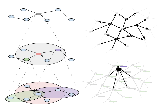
But if you have even a medium sized graph, this is really expensive, especially if you are doing it sequentially — it's N * D * M calculations, where N is the number of nodes, D is the average degree (number of connections) of each node, and M is the number of hops you want to aggregate over. This is part of the reason why a lot of early GNN work is done on molecules. The graph structure of a molecule is pretty small, so you could simply brute force your way through.
Graph representations
In order to solve the computational bottleneck we need to rethink how we represent our graph. This was always the hardest part of understanding graph learning for me, so I'm going to spend extra time on it. We're going to dive into a fair bit of the matrix implementation, but by the end we'll hopefully have a flexible model architecture that can handle a wide range of graph problems.
There are many ways to represent a graph. Naively, you could take the 'struct' approach and represent each node as an object that links out to other nodes. This is the format most preferred by leetcode enthusiasts, but it's basically never the right choice. A better approach is to represent the graph as an [N, N] matrix, where N is the number of nodes. Each value in the matrix i,j represents the strength of the connection from node i to node j. If the graph is bidirectional, the adjacency matrix is symmetric — that is, i,j will equal j,i.
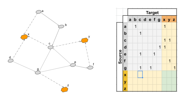
If you matmul the adjacency matrix A by a [N, Dnode] node embedding matrix, you can efficiently calculate an aggregation of node representations over a graph structure. And if you do this multiple times, you can calculate larger and larger representations.
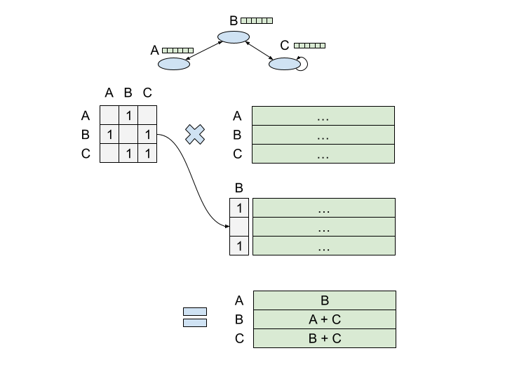
This is, roughly, what a Graph Convolutional Network (GCN) is doing. Hopefully you can see the parallels to actual convolutional networks — as you stack layers, you get a wider aperture on your input graph, exploiting the graph structure to determine what to pull in. Now, I have a special soft spot for these guys, in large part because I spent most of my time at Google training them5. But I also think these things are really elegant. In one shot, you calculate node representations for every node in the graph. No sequential processing required.
The adjacency matrix makes things computationally feasible, but GCNs don't really support edge features, and working with the adjacency matrix directly is still problematic over larger graphs — you have to load into memory a matrix of size N2. Can we make this more efficient? Well, in most graphs, the adjacency matrix is going to be mostly empty. There's just a ton of 0s because most nodes aren't connected to most other nodes6. We call this kind of matrix 'sparse', because data is 'sparsely' present throughout the matrix.
We can use a different representation to make our sparse matrix dense. Instead of having an NxN adjacency matrix, we can split our representation into three matrices:
A [E, Dedge] edge feature matrix, where each row represents the features associated with an edge
A [N, Dnode] node feature matrix, where each row represents the features associated with a given node.
A [2, E] index matrix, where each row is a [source, target] tuple that represents an edge between two nodes (source and target are numbers that are indices for nodes in the NxDnode matrix).
This representation only stores non-zero values, making the overall representation much smaller if the underlying graph is sparse78.
Architecture and experiments
In a fully general MPNN, we want to calculate a "message" from each node neighbor that is somehow transformed by edge features, compile all the messages that are being sent to a single node, and apply them to that node representation. The MPNN authors build on a variant called Gated Graph Neural Network (GG-NN) that takes advantage of sparse representations to efficiently to do all this.
We can use the index matrix to get all of the "source" node features [E, Dnode]. The same node features will be represented multiple times in this matrix, once per edge.
We can learn a basic MLP that takes in an edge feature and outputs a vector of size Dnode2. We can then reshape the output into an [E, Dnode, Dnode] tensor. The intuition here is that for each edge, we learn a transformation of the node features.
We matmul these two together. [E, Dnode, Dnode] * [E, Dnode] will output another [E, Dnode] matrix, which represents the "message" being "sent" by each node neighbor across a given edge.
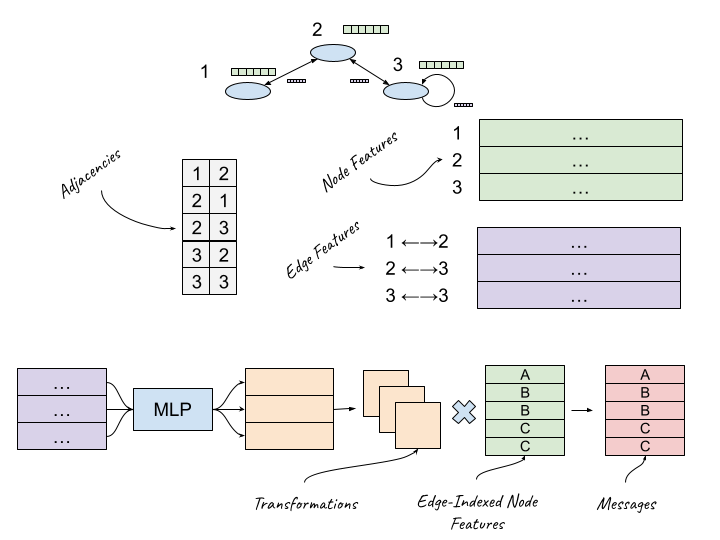
To compile the messages we add each message based on the target index in the index matrix9. And then we pass the summed message into a LSTM along with the previous representation.
So now we can zoom all the way back out to molecule production. The authors take a dataset with 130k molecules, each with molecular positions and properties about electron states and vibration frequences. And they take their architecture, and try and predict a set of quantum mechanical properties about each molecule based on the input. Since they are looking for predictions over the whole graph, they have a final step in the architecture where they take in all the node representations and collapse them into a single output value — they experiment with set2set, which we discussed previously here.
Experimental results
For the most part the results are what you'd expect, the model does reasonably well against some baselines. There's two interesting things that stand out.
First, the authors discuss ways to modify the underlying graph structure such that distant nodes can more easily influence each other10. In particular, the authors decide to create a single "master node" that is connected to every other node in the graph. The master node ingests messages from every other node in the graph at once, and then sends the same compiled message out to all other nodes.
Second, the authors discuss this weird multi tower structure, where instead of having one big model with a large feature dimension they create a set of M smaller models, each with an internal feature dimension of size D/M, which are then 'mixed' together using a neural net. Empirically this performs better, and it's faster. The authors theorize that this allows for a larger number of hidden states, though they do not really expand on this much at all.
Oof. Long paper. I think I might have failed at keeping this high level.
Insights
I spent a lot of time during my stint at Google thinking about graphs and graph learning. A lot of my intuition for ML models and representation learning came from thinking about graphs and graph representations. As a result I have a bunch of thoughts about this paper. Bear with me.
Graph structure is a hyperparameter
First, it's a bit interesting to talk about edge features. One natural way of representing graph data is to separate nodes and edges into separate categories of things. This naturally parallels how we talk about graphs in the real world — different nodes may have different kinds of connections that in turn signal different interactions. In the social network example, being friends is a different kind of connection than being blocked, but both of them are useful. The thought process behind learning a [D, D] edge transformation is, intuitively, aligned with the idea that the edge itself changes the underlying message. But the existence of edge features at all is a choice of graph construction. You can push all the features to the nodes on either end. More generally, the graph structure is a variable in itself, and can be modified in all sorts of ways before learning on it. The experiments with the "master node" come from the same basic intuition. This is part of what makes graph learning so interesting! You have a bunch more variables in your problem set up that you can play with.
Building on the above, it turns out that you can adjust your problem statement to make things much more scalable. Instead of training on an entire graph simultaneously, you can load patches of the graph at a time and train only on those patches. You can scale this to run in parallel across a bunch of machines, such that at any given time you can train a pretty large effective batch size11. We did this a lot at Google, where graphs would regularly have billions of nodes.
Towers as regularization
The first time I read this paper, I didn't understand the point of those towers at all. It always seemed strictly worse to me. If you have a model with an internal feature representation of size D, the number of possible interactions between dimensions is D2. Or, put another way, a model's representation capacity increases proportional to the square of the feature dimension. By cutting each tower into N pieces, you get a model capacity that is proportional to sumN( (D/N)2 ). Which, of course, is less than D2.
But after reading a few more of these papers, I think the empirical improvement makes a bit more sense. These towers are a form of model regularization, as well as a form of attention head. Each tower likely learns a different, specialized function. I don't know if many folks really use this multi-tower structure in 2024/5, I suspect you can get the same results by just increasing other forms of regularization. But I'd be curious, from an interpretability perspective, to know if the same towers have different [D, D] edge transformation matrices or meaningfully different node representations. More generally, I think there's likely a parallel between having multiple convolution filters, having multiple transformer attention heads, and having multiple GNN towers.
GNNs generalize convolutions
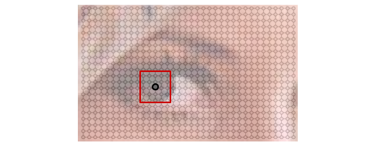
I and others have previously written that convolutional networks learn to exploit geometric relationships in images. Pixels near each other are grouped and analyzed together, resulting in increasingly lower resolution windows that are correspondingly "richer" in their representations. One way to model an image is as a graph, where each pixel is a node with a three dimensional feature vector representing RGB, and with edges between every pixel and its neighbors.
When we spoke about semantic segmentation in my review of the Dilated Convolution paper, I said
Back in 2016, there had been a bunch of progress on image classification, and deep learning models were far and away the best automated classifiers. The same could not be said for image segmentation. The former is about taking an image and deciding what category it should be in. It is, fundamentally, a bucketing problem. The latter is about taking an image and deciding which pixels correspond to which objects. This is significantly harder.
…
Classification is all about decreasing resolution. You start with a HxWx3 input vector (an RGB image) and need to reduce the resolution down to a vector with D categories. So you can use pooling and subsampling layers. At each resolution decrease step, you only need to retain the important information for the classifier at the end; you can throw away anything else.
But with semantic segmentation, you can't reduce the resolution — you have to keep the pixel level information in the model all the way through to the end, to be able to output pixel masks — but you also have to reduce the resolution in order to get an understanding of where the hotdog starts and ends. Your model needs to somehow compile all of the information of the image, and apply its understanding of the image to each pixel separately.
Graph learning also has a separation between classification and "segmentation". The former is a bit obvious — can we learn some properties (categories) about the overall graph? This is what the authors of this paper are interested in, and why they have a "graph readout" step in their architecture. That's roughly the equivalent of a pooling step in a traditional convolution.
As for the latter, in a lot of graph learning problems, you want to learn how to label nodes, so you build up a representation for each node and categorize each one separately. Semantic segmentation is a type of node classification task — your nodes are pixels, your classes are object-mask membership.
GNNs generalize RNNs
An RNN is used to process sequences. At each step in a sequence, the RNN ingests some data and it's own previous state, and optionally outputs some value. Often, the sequence is modeled as a "temporal" one — we model the steps in the sequence using t, and we call the whole structure "back propagation through time".
But you can model the same setup as a graph with no loss of generality. A sequence is a graph in which each node is an element of the sequence, with a one-directional edge to the next element in the sequence. A bit like a linked list. At each node, you calculate a "message" that gets sent to the next node in the graph. If your sequence is size S, you can model an RNN as a graph neural network that aggregates messages over S steps.

In the MPNN paper, the authors discuss "weight tying". This is a hyperparameter that determines whether each step of the model uses the same weights, or uses different weights. An MPNN with weight tying is essentially equivalent to an actual RNN, which uses the same weights at each "timestep" of the sequence it is running on.
Attention and GNNs
Graph Neural Networks have to be invariant to the ordering and labeling of graph nodes. In other words, they have to treat every layer as a set instead of a sequence. In a previous review, we discussed how attention is an order invariant operation. As it turns out, attention and MPNNs are really closely related.
To recap, the basic idea behind attention in language modeling is to learn how each previous word in a sentence relates to the current word being analyzed. This is almost always implemented as a weighted sum of word vectors. The weights are scalars that are output by some similarity function on the source and target word vectors, either a learned network or a simple matmul (cosine similarity).
One way to think about attention is that you are trying to learn a set of adjacency weights in a graph. Each word is a node, and the weights are the strengths of the edge connections between nodes. Each word is "sending a message" to all of the other words. The message is modulated in strength and direction by the edge weight.
You can flip this around too. One way to think of the MPNN is you are learning how to combine data given a fixed attention matrix provided as input in the form of a graph. Each edge transformation is a simple generalization of the edge weight discussed above.
Self attention (e.g. in transformers) is especially closely related to the GCN implementation we discussed above. Transformers explicitly learn and materialize a QK attention matrix, which can be thought of as an [N, N] adjacency matrix of every word-node in a sentence-graph to every other word-node. In a GCN, you multiply your graph adjacency matrix by your node features matrix to get a weighted neighborhood representation. In a transformer, you multiply your "attention" matrix by your V matrix to transform each word vector by every other word vector. These are exactly equivalent operations; it's just that in the GCN the graph is provided by some external source instead of some internal, learned one.
No wonder transformers are so powerful — their primary representational unit is one of the most expressive data structures in mathematics!
In my opinion, this relationship is very cool. It suggests that some of the ways in which we scale GNNs may be applicable to transformers, which are primarily limited by the N2 computational complexity of the attention matrix. It also gives us a way to reason about what transformers are doing — we can initialize the word graphs associated with each attention head and manually inspect how they relate. Finally, it makes me wonder about the sparsity difference between attention matrices and graph matrices. Can you make transformers sparse without losing capacity? Or are transformers generally learning very dense graphs?
I think these reviews are getting longer with each paper, oops. That said, I'm enjoying really digging into the connections across all of them.
And, in fact, until AlphaFold 2 in 2020, the former was considered one of the biggest unsolved problems in chemistry and biology, so much so that Demis Hassabis won the Nobel Prize this year on the back of DeepMind's work.
Actually, in some cases, we're explicitly trying to learn a good graph representation!
Which is a very reasonable assumption — generally graphs represent some connection that matters in the real world, like friendships or transactions.
Sums are transitive — order doesn't matter — and they act as a reduce operation, allowing for 'different scales' of input.
And may have the claim to being the first person at Google to ever train one of these internally!
As an intuition pump, think about facebook. Most people probably have a few hundred friends on facebook, but there are literally billions of monthly active users. The full graph adjacency matrix is almost entirely empty values.
There is a slight overhead because we have to represent the edges in a separate vector. In dense matrices, you wouldn't want to use this implementation — it would take up extra space.
This also isn't the only way to represent a sparse matrix, but it works well for graphs.
I'm not going to get too deep into how this is done, but take a look at the scatter_add op.
In the molecule case, you could imagine two atoms that are physically close to each other and interact due to their magnetic properties, but are on opposite ends of a graph representation of the molecule.
Though, granted, this is still an approximation over training on the entire graph.


